Example 06 – Cross sections & flux uncertainties

Aims

• Turn cross sections as input parameters into event numbers using fluxes

• Implement flux uncertainties

Instructions

So far we have concentrated on raw event numbers or simple template scaling parameters to parameterize the number of events we expect to see in our detector. But these raw numbers or templates themselves depend on other more fundamental parameters.

E.g, if you are recording products of a radioactive decay, they will depend on the number of radioactive nuclei inside the detector, the decay rates into the different states you are distinguishing, and the total amount of time the experiment was collecting data:

n_true_events_in_state_j = N_nuclei * time * decay_rate_to_state_j

Of these three parameters, the decay rate is usually the truly interesting one. It is the physics one wants to examine with the experimental setup. The number of nuclei and the time that the experiment ran on the other hand are just properties of the experimental setup and the data that was recorded. So just like the detector response, it would be good if we could absorb them into a Predictor, so that we can do statistical tests with the interesting physics parameters directly.

A slightly more complicated example is the measurement of interactions of a particle beam with a target material, e.g. a neutrino beam with a water target. Here the number of true events depends and the neutrino flux as a function of the neutrino energy, the number of target molecules in the detector, and the neutrino interaction cross sections for the different final states distinguished by the detector:

n_true_events_j = T * sum_k(sigma_jk * F_k)

Here T is the number of targets, F_k is the integrated recorded neutrino flux in neutrino energy bin k (unit: neutrinos/m^2), and sigma_jk is the cross section for neutrinos in energy bin k to cause a reaction to the final state j that can be recorded by the detector.

In general, a lot of experimental setups can be described with a matrix multiplication in the form:

n_true_events_j = sum_k(physics_parameter_matrix_jk * exposure_k)

Depending on the details of the experiment, the parameter matrix and exposure vector have slightly different meanings. In the case of the radioactive decay measurement, the physics parameters would be the decay rates, and the exposure would be the product of number of nuclei and the recording time. In the neutrino case the parameters would be the cross sections, and the exposure would be the product of integrated neutrino fluxes and target mass. In the context of a collider experiment, the exposure would probably be called an integrated luminosity.

We will extend the previous example and treat it like a neutrino beam experiment. First we will need to get the binning in the true event properties:

import numpy as np
import pandas as pd

from remu import binning

with open("../05/truth-binning.yml") as f:
    truth_binning = binning.yaml.full_load(f)

# Get truth binnings for BG and signal
bg_truth_binning = truth_binning.subbinnings[1].clone()
signal_truth_binning = truth_binning.subbinnings[2].clone()

As a binning for the flux, we will use a simple linear binning in the neutrino energy:

!LinearBinning
bin_edges:
- 0.0
- 2.0
- 4.0
- 6.0
- 8.0
- 10.0
- 12.0
- 16.0
- 20.0
- .inf
include_upper: false
phasespace: !PhaseSpace
- E
variable: E

# Define flux binning
with open("flux-binning.yml") as f:
    flux_binning = binning.yaml.full_load(f)

The binning of the cross section is done as a CartesianProductBinning. Every possible combination of true kinematic bin and true neutrino energy bin gets its own cross-section values:

# Create cross-section binnings
bg_flux_binning = flux_binning.clone()
bg_xsec_binning = binning.CartesianProductBinning((bg_truth_binning, bg_flux_binning))
signal_flux_binning = flux_binning.clone()
signal_xsec_binning = binning.CartesianProductBinning(
    (signal_truth_binning, signal_flux_binning)
)

We can have a look at the structure of the resulting binning:

# Check binning structure
n_bg_truth = bg_truth_binning.data_size
n_signal_truth = signal_truth_binning.data_size
n_flux = flux_binning.data_size
n_bg_xsec = bg_xsec_binning.data_size
n_signal_xsec = signal_xsec_binning.data_size
print(n_bg_truth, n_signal_truth, n_flux)
print(n_bg_xsec, n_signal_xsec)
print(signal_xsec_binning.bins[0].data_indices)
print(signal_xsec_binning.bins[1].data_indices)
print(signal_xsec_binning.bins[n_flux].data_indices)

48 120 9
432 1080
(0, 0)
(0, 1)
(1, 0)

An increase of the bin index by one means that we increase the corresponding data index in the flux binning by one. Once every flux bin has been stepped through, the data index in the truth binning increases by one.

To create a Predictor that can turn cross sections into event numbers, we need an actual neutrino flux. We can easily create one by filling the flux binning:

# Fill flux with exposure units (proportional to neutrinos per m^2)
from remu import plotting
from numpy.random import default_rng

rng = default_rng()
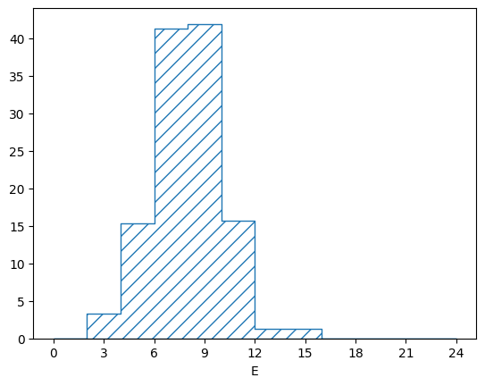
E = rng.normal(loc=8.0, scale=2.0, size=1000)
df = pd.DataFrame({"E": E})
flux_binning.fill(df, weight=0.01)

We fill the binning with a weight of 0.01 so that the total amount of exposure in the binning is 10, corresponding with the assumed 10 years of data taking used for the event generation in the previous examples. So one “unit” of exposure corresponds to one year of data taking.

The “simulated” flux looks like this:

pltr = plotting.get_plotter(flux_binning)
pltr.plot_values()
pltr.savefig("flux.png")

Of course the exact flux is never known (especially with neutrino experiments). To simulate a flux uncertainty, we can just create lots of throws:

# Create fluctuated flux predictions
E_throws = rng.normal(loc=8.0, scale=2.0, size=(100,1000))
flux = []
for E in E_throws:
    df = pd.DataFrame({"E": E})
    flux_binning.reset()
    flux_binning.fill(df, weight=0.01)
    flux.append(flux_binning.get_values_as_ndarray())

flux = np.asfarray(flux)
print(flux.shape)

(100, 9)

Now we can use those flux predictions to create a LinearEinsumPredictor that will do the correct matrix multiplication to combine the cross sections and the flux into event numbers:

# Create event number predictors
from multiprocess import Pool
from remu import likelihood
pool = Pool(8)
likelihood.mapper = pool.map

bg_predictor = likelihood.LinearEinsumPredictor(
    "ij,...kj->...ik",
    flux,
    reshape_parameters=(n_bg_truth, n_flux),
    bounds=[(0.0, np.inf)] * bg_xsec_binning.data_size,
)
signal_predictor = likelihood.LinearEinsumPredictor(
    "ij,...kj->...ik",
    flux,
    reshape_parameters=(n_signal_truth, n_flux),
    bounds=[(0.0, np.inf)] * signal_xsec_binning.data_size,
)

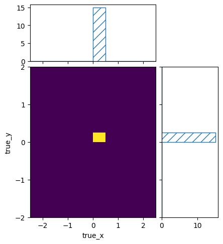
Let us do a quick test of the predictions:

# Test cross-section predictions
signal_xsec_binning.reset()
signal_xsec_binning.fill({"E": 8.0, "true_x": 0.0, "true_y": 0.0}, 100.0)
signal_xsec = signal_xsec_binning.get_values_as_ndarray()

signal_events, weights = signal_predictor(signal_xsec)
signal_truth_binning.set_values_from_ndarray(signal_events)
pltr = plotting.get_plotter(signal_truth_binning)
pltr.plot_values(density=False)
pltr.savefig("many_events.png")

signal_xsec_binning.reset()
signal_xsec_binning.fill({"E": 3.0, "true_x": 0.0, "true_y": 0.0}, 100.0)
signal_xsec = signal_xsec_binning.get_values_as_ndarray()

signal_events, weights = signal_predictor(signal_xsec)
signal_truth_binning.set_values_from_ndarray(signal_events)
pltr = plotting.get_plotter(signal_truth_binning)
pltr.plot_values(density=False)
pltr.savefig("few_events.png")

Despite filling the same cross section to the same true kinematics int the two cases, the resulting number of events was different. This is of course because the flux at 3 is smaller than the flux at 8. So even if the cross sections at 3 and 8 are the same, the different flux will lead to a different number of predicted events.

Finally we need a predictor for the noise events. These are events that do not correspond to any interesting physics and are just weighted up or down with a single parameter as input to the response matrix, so we will just pass through that single parameter. We will use the TemplatePredictor for this, since it set the parameter limits to (0, np.inf) by default, which is convenient here. In order or the systematics to line up, we will have to create 100 identical “variations”:

# Create noise predictor
noise_predictor = likelihood.TemplatePredictor([[[1.0]]] * 100)

Now that we have the three separate predictors for the noise, background, and signal events, we need to combine them into a single ConcatenatedPredictor:

# Combine into single predictor
event_predictor = likelihood.ConcatenatedPredictor(
    [noise_predictor, bg_predictor, signal_predictor],
    combine_systematics="same"
)

The input of the combined predictor will be a concatenation of the separate inputs. I.e. first the single noise scaling parameter, then the background cross-section parameters, and finally the signal cross-section parameters. The output likewise will be a concatenation of the single output: first the unmodified noise scaling parameter, then the background events numbers, and finally the signal event numbers. If we have done everything right, this corresponds exactly to the meaning of the data of the original truth_binning, so it can be used as input for the response matrix.

At this point we could combine the event predictor with a response matrix and likelihood calculator to do statistical tests with the cross-section parameters. With hundreds or thousands of parameters, this is a computationally intensive task though. So for this tutorial we will again define some models as templates and investigate them by varying their weights.

In order to to simplify that task, we will first create a binning that encapsulates all input parameters for the event_predictor:

parameter_binning = truth_binning.marginalize_subbinnings()
parameter_binning = parameter_binning.insert_subbinning(1, bg_xsec_binning)
parameter_binning = parameter_binning.insert_subbinning(2, signal_xsec_binning)

We started by marginalizing out all subbinnings in the original truth_binning, which yield a binning that only distinguishes the three event types in order: noise, background, signal. Then we inserted the cross-section binnings as subbinnings into their respective top level bins. This leaves us with a binning where the desired data structure: first a single bin for the noise, then the background cross-section bins as defined by the bg_xsec_binning, and finally the signal cross-section bins as defined by signal_xsec_binning.

The template for the noise events is simple. Again, we just want to scale the noise parameter directly:

noise_template = np.zeros(parameter_binning.data_size)
noise_template[0] = 1.0

For the cross-section templates, we need to take a look at the cross-section bins, so we can understand what values to put in them:

for i, b in enumerate(bg_xsec_binning.bins):
    # Get truth and flux bin from Cartesian Product
    truth_bin, flux_bin = b.get_marginal_bins()

    print(i)
    print(truth_bin)
    print(flux_bin)

    break

0
RectangularBin(include_upper=False, include_lower=True, variables=['true_x', 'true_y'], edges=[[-inf, -0.5], [-inf, -0.25]], phasespace=PhaseSpace(variables={'true_x', 'true_y'}), value_array=array([0.]), entries_array=array([0]), sumw2_array=array([0.]))
RectangularBin(include_upper=False, include_lower=True, variables=['E'], edges=[[0.0, 2.0]], phasespace=PhaseSpace(variables={'E'}), value_array=array([0.]), entries_array=array([0]), sumw2_array=array([0.]))

The method CartesianProductBin.get_marginal_bins() returns the bins of the original binnings, that correspond to the given bin of the CartesianProductBinning. In this case, these are the bin of the true kinematics, and the bin of the neutrino Energy. For each we have the edges of the bin, so we can use those to calculate the correct cross section: The number of true events expected in the given truth bin, for each unit of exposure in the given flux bin:

from scipy.stats import expon, norm, uniform


def calculate_bg_xsec(E_min, E_max, x_min, x_max, y_min, y_max):
    """Calculate the cross section for the BG process."""

    # We need to make an assumption about the E dsitribution within the E bin
    # Bin edges can be +/- np.inf
    if np.isfinite(E_min) and np.isfinite(E_max):
        # Uniform in given bounds
        E_dist = uniform(loc=E_min, scale=E_max - E_min)
    elif np.isfinite(E_min):
        # Exponential from E_min to inf
        E_dist = expon(loc=E_min)
    else:
        # Exponential from -inf to E_max
        E_dist = expon(loc=E_max, scale=-1)

    # Simple overall cross section: One unit of exposure yields 30 true events
    xsec = 30.0

    # True x is True E with a shift and scale
    # Average XSEC in bin is proportional to overlap
    E_0 = (x_min - 0.5) * 2 / np.sqrt(0.5) + 8
    E_1 = (x_max - 0.5) * 2 / np.sqrt(0.5) + 8
    lower = max(E_min, E_0)
    upper = min(E_max, E_1)
    if upper >= lower:
        xsec *= E_dist.cdf(upper) - E_dist.cdf(lower)
    else:
        xsec = 0.0

    # Differential XSEC in y is Gaussian
    # Independent of x
    y_dist = norm(loc=0.5, scale=np.sqrt(0.5))
    xsec *= y_dist.cdf(y_max) - y_dist.cdf(y_min)

    return xsec


bg_template = np.zeros(parameter_binning.data_size)
bg_xsec = np.zeros(bg_xsec_binning.data_size)
bg_offset = parameter_binning.get_bin_data_index(1)
for i, b in enumerate(bg_xsec_binning.bins):
    # Get truth and flux bin from Cartesian Product
    truth_bin, flux_bin = b.get_marginal_bins()

    E_min, E_max = flux_bin.edges[0]
    x_min, x_max = truth_bin.edges[0]
    y_min, y_max = truth_bin.edges[1]

    bg_xsec[i] = calculate_bg_xsec(E_min, E_max, x_min, x_max, y_min, y_max)
    bg_template[i + bg_offset] = bg_xsec[i]

pltr = plotting.get_plotter(bg_xsec_binning)
pltr.plot_array(bg_xsec)
pltr.savefig("bg_xsec.png")

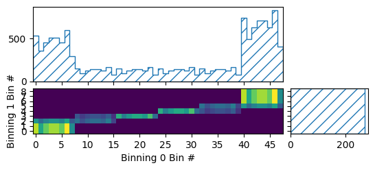
This plot of the template is not very intuitive, since the plotter of a general CartesianProductBinning does not know the meaning of the single bins in the constituent binnings. So it can only plot bin numbers vs one another. A CatesianProductBinning consisting of only RectilinearBinning, and LinearBinning without any subbinnings has the same data structure as a RectilinearBinning though, so we can use that plotter to get a slightly more readable plot:

bg_xsec_plot_binning = binning.RectilinearBinning(
    bg_truth_binning.variables + (flux_binning.variable,),
    bg_truth_binning.bin_edges + (flux_binning.bin_edges,),
)
pltr = plotting.get_plotter(bg_xsec_plot_binning)
pltr.plot_array(bg_xsec, density=[0, 1], hatch=None)
pltr.savefig("bg_xsec_pretty.png")

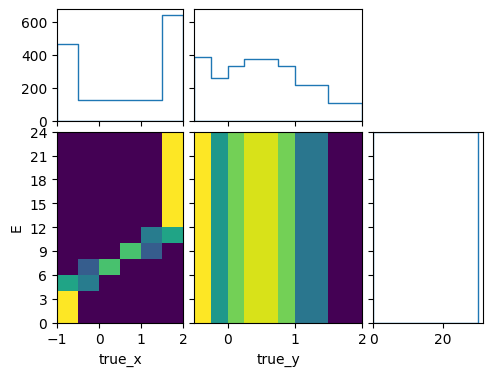
Here we told the plotter to only plot densities with relation to variables 0 and 1, i.e. true_x and true_y. This means the plots are “differential” in true_X and true_y but not in E. The marginal plot of the E “distribution” shows the total cross section of each bin, and not a density. The marginal plots of true_x and true_y are technically differential cross sections, but in this particular case they are flux integrated over a flux with one unit of exposure in each energy bin. In order to see the flux integrated cross sections in the actual flux, we need to use the predictors to actually predict the number of events:

bg_truth_binning.reset()
bg_truth_binning.fill_from_csv_file("../05/bg_truth.txt", weight=0.1)
pltr = plotting.get_plotter(bg_truth_binning)
pltr.plot_values(scatter=500, label="generator")

bg_pred, w = bg_predictor(bg_xsec)
pltr.plot_array(bg_pred, scatter=500, label="xsec")

pltr.legend()
pltr.savefig("bg_prediction.png")

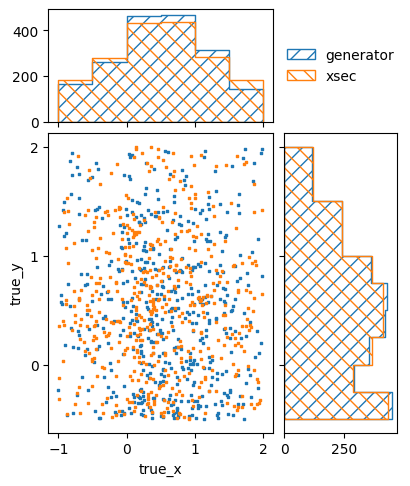
Here we also plotted the previously generated number of events for comparison. The prediction from the cross-section model is not a perfect match, but it is very close.

Now that we have a cross section for the background process, we need to repeat this process for the two signal processes:

def calculate_model_A_xsec(E_min, E_max, x_min, x_max, y_min, y_max):
    """Calculate the cross section for the model A process."""

    # We need to make an assumption about the E dsitribution within the E bin
    # Bin edges can be +/- np.inf
    if np.isfinite(E_min) and np.isfinite(E_max):
        # Uniform in given bounds
        E_dist = uniform(loc=E_min, scale=E_max - E_min)
    elif np.isfinite(E_min):
        # Exponential from E_min to inf
        E_dist = expon(loc=E_min)
    else:
        # Exponential from -inf to E_max
        E_dist = expon(loc=E_max, scale=-1)

    # Simple overall cross section: One unit of exposure yields 100 true events
    xsec = 100.0

    # True x is True E with a shift and scale
    # Average XSEC in bin is proportional to overlap
    E_0 = (x_min - 0.1) * 2.0 + 8
    E_1 = (x_max - 0.1) * 2.0 + 8
    lower = max(E_min, E_0)
    upper = min(E_max, E_1)
    if upper >= lower:
        xsec *= E_dist.cdf(upper) - E_dist.cdf(lower)
    else:
        xsec = 0.0

    # Differential XSEC in y is Gaussian
    # Independent of x
    y_dist = norm(loc=0.2, scale=1.0)
    xsec *= y_dist.cdf(y_max) - y_dist.cdf(y_min)

    return xsec


model_A_xsec = np.zeros(signal_xsec_binning.data_size)
model_A_template = np.zeros(parameter_binning.data_size)
signal_offset = parameter_binning.get_bin_data_index(2)
for i, b in enumerate(signal_xsec_binning.bins):
    # Get truth and flux bin from Cartesian Product
    truth_bin, flux_bin = b.get_marginal_bins()

    E_min, E_max = flux_bin.edges[0]
    x_min, x_max = truth_bin.edges[0]
    y_min, y_max = truth_bin.edges[1]

    model_A_xsec[i] = calculate_model_A_xsec(E_min, E_max, x_min, x_max, y_min, y_max)
    model_A_template[i + signal_offset] = model_A_xsec[i]

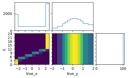
signal_xsec_plot_binning = binning.RectilinearBinning(
    signal_truth_binning.variables + (flux_binning.variable,),
    signal_truth_binning.bin_edges + (flux_binning.bin_edges,),
)
pltr = plotting.get_plotter(signal_xsec_plot_binning)
pltr.plot_array(model_A_xsec, density=[0, 1], hatch=None)
pltr.savefig("model_A_xsec.png")

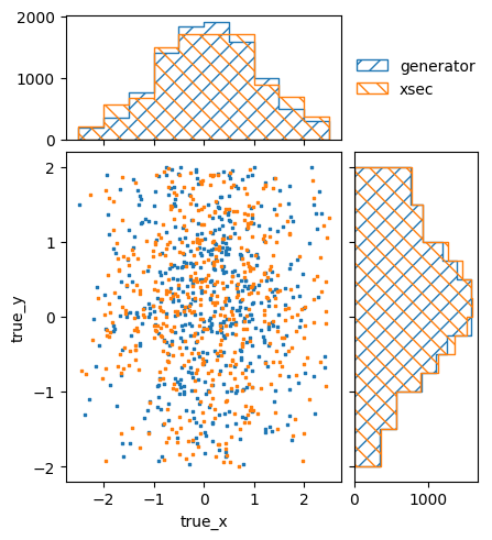
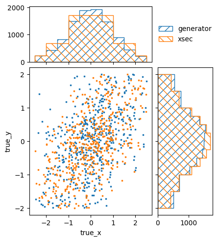
signal_truth_binning.reset()
signal_truth_binning.fill_from_csv_file("../00/modelA_truth.txt", weight=0.1)
pltr = plotting.get_plotter(signal_truth_binning)
pltr.plot_values(scatter=500, label="generator")

model_A_pred, w = signal_predictor(model_A_xsec)
pltr.plot_array(model_A_pred, scatter=500, label="xsec")

pltr.legend()
pltr.savefig("model_A_prediction.png")

model_B_xsec = np.zeros(signal_xsec_binning.data_size)
model_B_template = np.zeros(parameter_binning.data_size)
signal_offset = 1 + bg_xsec_binning.data_size


def calculate_model_B_xsec(E_min, E_max, x_min, x_max, y_min, y_max):
    """Calculate the cross section for the model A process."""

    # We need to make an assumption about the E dsitribution within the E bin
    # Bin edges can be +/- np.inf
    if np.isfinite(E_min) and np.isfinite(E_max):
        # Uniform in given bounds
        E_dist = uniform(loc=E_min, scale=E_max - E_min)
    elif np.isfinite(E_min):
        # Exponential from E_min to inf
        E_dist = expon(loc=E_min)
    else:
        # Exponential from -inf to E_max
        E_dist = expon(loc=E_max, scale=-1)

    # Simple overall cross section: One unit of exposure yields 100 true events
    xsec = 100.0

    # True x is True E with a shift and scale
    # Average XSEC in bin is proportional to overlap
    E_0 = (x_min - 0.0) * 2.0 + 8
    E_1 = (x_max - 0.0) * 2.0 + 8
    lower = max(E_min, E_0)
    upper = min(E_max, E_1)
    if upper >= lower:
        xsec *= E_dist.cdf(upper) - E_dist.cdf(lower)
    else:
        xsec = 0.0

    # Differential XSEC in y is Gaussian
    # Correalted with x
    # Should integrate 2D distribution of x/E and y
    # Instead, cheat and assume median E value
    if np.isfinite(lower) and np.isfinite(upper):
        E_m = (upper + lower) / 2
    elif np.isfinite(lower):
        E_m = lower + 1
    elif np.isfinite(upper):
        E_m = upper - 1
    else:
        E_m = 0.0
    x_m = (E_m - 8.0) / 2

    y_dist = norm(loc=0.5 * x_m, scale=1.0 - 0.5**2)
    xsec *= y_dist.cdf(y_max) - y_dist.cdf(y_min)

    return xsec


for i, b in enumerate(signal_xsec_binning.bins):
    # Get truth and flux bin from Cartesian Product
    truth_bin, flux_bin = b.get_marginal_bins()

    E_min, E_max = flux_bin.edges[0]
    x_min, x_max = truth_bin.edges[0]
    y_min, y_max = truth_bin.edges[1]

    model_B_xsec[i] = calculate_model_B_xsec(E_min, E_max, x_min, x_max, y_min, y_max)
    model_B_template[i + signal_offset] = model_B_xsec[i]

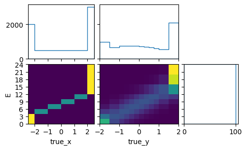
pltr = plotting.get_plotter(signal_xsec_plot_binning)
pltr.plot_array(model_B_xsec, density=[0, 1], hatch=None)
pltr.savefig("model_B_xsec.png")

signal_truth_binning.reset()
signal_truth_binning.fill_from_csv_file("../00/modelB_truth.txt", weight=0.1)
pltr = plotting.get_plotter(signal_truth_binning)
pltr.plot_values(scatter=500, label="generator")

model_B_pred, w = signal_predictor(model_B_xsec)
pltr.plot_array(model_B_pred, scatter=500, label="xsec")

pltr.legend()
pltr.savefig("model_B_prediction.png")

Now that we have the templates, we can combine them into a TemplatePredictor:

# Template predictor for noise, bg, model A, model B
xsec_template_predictor = likelihood.TemplatePredictor(
    [noise_template, bg_template, model_A_template, model_B_template]
)

This can then be combined with the detector response and event predictor to get the full chain to the reconstructed level:

# Load data and response matrix

with open("../01/reco-binning.yml") as f:
    reco_binning = binning.yaml.full_load(f)

reco_binning.fill_from_csv_file("../05/real_data.txt")
data = reco_binning.get_entries_as_ndarray()
data_model = likelihood.PoissonData(data)

response_matrix = "../05/response_matrix.npz"
matrix_predictor = likelihood.ResponseMatrixPredictor(response_matrix)

# Combine into linear predictor
data_predictor = likelihood.ComposedPredictor(
    [matrix_predictor, event_predictor],
    combine_systematics="same",
)
template_predictor = likelihood.ComposedMatrixPredictor(
    [data_predictor, xsec_template_predictor], combine_systematics="cartesian"
)

We composed the matrix_predictor and event_predictor with the same strategy for combining systematics. This means that the 100 flux variations are matched one-to-one to the 100 detector response variations, for a total of 100 systematic variations. The default cartesian strategy would man that each of the 100 detector variations is combined with all of the 100 flux variations, for a total of 10,000 systematic variations.

For the final template_predictor we compose the data_predictor and xsec_template_predictor using a ComposedMatrixPredictor. This is a special kind of ComposedPredictor, which pre-computes a linear approximation of the composed predictors in the form of a matrix multiplication. So for a prediction, it does _not_ need to call the original predictors in order, but only needs to do a simple matrix multiplication, where the matrix is the size of the number of output parameters times the number of input parameters. This speeds things up considerably, since we effectively circumvent the hundreds of cross-section parameters that would otherwise need to be calculate each time the predictor is called. And since all predictors that go into this final predictor are actually linear, the linear “approximation” is actually exact (modulo numerical variations).

Now that we have a performant predictor of the reconstructed data, we can run statistical analyses with it, like a simple maximum likelihood fit:

# Likelihood caclulator and hypothesis tester
calc = likelihood.LikelihoodCalculator(data_model, template_predictor)
maxi = likelihood.BasinHoppingMaximizer()

# Fit everything
ret = maxi.maximize_log_likelihood(calc)
print(ret)

                        fun: 27.15065583063253
             log_likelihood: -27.15065583063253
 lowest_optimization_result:       fun: 27.15065583063253
 hess_inv: <4x4 LbfgsInvHessProduct with dtype=float64>
      jac: array([4.61852412e-06, 8.63309424e-05, 2.69738365e-01, 2.86348724e-04])
  message: 'CONVERGENCE: REL_REDUCTION_OF_F_<=_FACTR*EPSMCH'
     nfev: 250
      nit: 35
     njev: 50
   status: 0
  success: True
        x: array([239.81428165,   0.3976332 ,   0.        ,   1.08239838])
                    message: ['requested number of basinhopping iterations completed successfully']
      minimization_failures: 0
                       nfev: 1045
                        nit: 10
                       njev: 209
                    success: True
                          x: array([239.81428165,   0.3976332 ,   0.        ,   1.08239838])

We can calculate the overall p-values for the two hypotheses:

# Calculate p-values for hypotheses overall
calc_A = calc.fix_parameters([None, None, None, 0.0])
calc_B = calc.fix_parameters([None, None, 0.0, None])
test_A = likelihood.HypothesisTester(calc_A)
test_B = likelihood.HypothesisTester(calc_B)
print(test_A.max_likelihood_p_value())
print(test_B.max_likelihood_p_value())

0.6
0.86

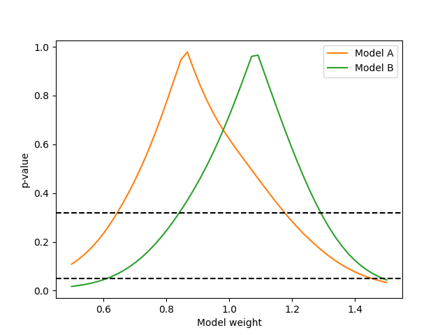
Or we can do a scan of the Wilks p-value for the model template weights:

# Get Wilks' p-values for models
norms = np.linspace(0.5, 1.5, 50)
p_values_A = []
p_values_B = []
for n in norms:
    p_values_A.append(test_A.wilks_max_likelihood_ratio_p_value([None, None, n]))
    p_values_B.append(test_B.wilks_max_likelihood_ratio_p_value([None, None, n]))

from matplotlib import pyplot as plt

fig, ax = plt.subplots()
ax.set_xlabel("Model weight")
ax.set_ylabel("p-value")
ax.plot(norms, p_values_A, label="Model A", color="C1")
ax.plot(norms, p_values_B, label="Model B", color="C2")
ax.axhline(0.32, color="k", linestyle="dashed")
ax.axhline(0.05, color="k", linestyle="dashed")
ax.legend(loc="best")
fig.savefig("wilks-p-values.png")

Since the flux integrations and uncertainty is now handled by the predictors, the cross-section parameters (or templates of cross-section parameters) can be used just like described in the previous examples.