Example 03 – Detector uncertainties

Aims

• Generate random detector response variations

• Include detector uncertainties in the response matrix by using a ResponseMatrixArrayBuilder

• Include statistical uncertainties by generating randomly varied matrices

• Use varied response matrices for fits and hypothesis tests

Instructions

The properties of experimental setups are usually only known to a finite precision. The remaining uncertainty on these properties, and thus the uncertainty on the detector response to true events, must be reflected in the response matrix.

We can create an event-by-event variation of the detector response with the provided script:

$ ../simple_experiment/vary_detector.py ../00/modelA_data.txt modelA_data.txt
$ ../simple_experiment/vary_detector.py ../00/modelB_data.txt modelB_data.txt

It creates 100 randomly generated variations of the simulated detector and varies the simulation that was created in example 00 accordingly. Each variation describes one possible real detector and is often called a “toy variation” or a “universe”.

Events are varied in two ways: The values of reconstructed variables can be different for each toy, and each event can get assigned a weight. The former can be used to cover uncertainties in the detector precision and accuracy, while the latter is a simple way to deal with uncertainties in the overall probability of reconstructing an event.

In this case, the values of the reconstructed reco_x are varied and saved as reco_x_0 to reco_x_99. The detection efficiency is also varied and the ratio of the events nominal efficiency and the efficiency assuming the toy detector stored as weight_0 up to weight_99. Let us plot the different reconstructed distributions we get from the toy variations:

import numpy as np

from remu import binning, plotting

with open("../01/reco-binning.yml") as f:
    reco_binning = binning.yaml.full_load(f)

# Get real data
reco_binning.fill_from_csv_file("../00/real_data.txt")
data = reco_binning.get_values_as_ndarray()

# Get toys
n_toys = 100
toyA = []
toyB = []
for i in range(n_toys):
    reco_binning.reset()
    reco_binning.fill_from_csv_file(
        "modelA_data.txt",
        weightfield="weight_%i" % (i,),
        rename={"reco_x_%i" % (i,): "reco_x"},
        buffer_csv_files=True,
    )
    toyA.append(reco_binning.get_values_as_ndarray())

    reco_binning.reset()
    reco_binning.fill_from_csv_file(
        "modelB_data.txt",
        weightfield="weight_%i" % (i,),
        rename={"reco_x_%i" % (i,): "reco_x"},
        buffer_csv_files=True,
    )
    toyB.append(reco_binning.get_values_as_ndarray())

# Plot
pltr = plotting.get_plotter(reco_binning)
for A, B in zip(toyA, toyB):
    pltr.plot_array(A / 10.0, alpha=0.05, edgecolor="C1", hatch=None)
    pltr.plot_array(B / 10.0, alpha=0.05, edgecolor="C2", hatch=None)

A = np.mean(toyA, axis=0)
B = np.mean(toyB, axis=0)
pltr.plot_array(data, label="Data", hatch=None, edgecolor="C0", linewidth=2)
pltr.plot_array(A / 10.0, label="Model A", hatch=None, edgecolor="C1")
pltr.plot_array(B / 10.0, label="Model B", hatch=None, edgecolor="C2")
pltr.legend()
pltr.savefig("data.png")

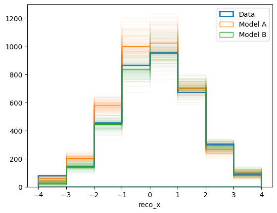
Here we simply plot one histogram for each toy data set with a low alpha value (i.e with high transparency), as well as a solid histogram for the mean values. Also we scaled the model predictions by a factor 10, simply because that makes “experiment running time” of the model predictions correspond to the data.

We are using a few specific arguments to the fill_from_csv_file method:

weightfield

Tells the object which field to use as the weight of the events. Does not need to follow any naming conventions. Here we tell it to use the field corresponding to each toy.

rename

The binning of the response matrix expects a variable called reco_x. This variable is not present in the varied data sets. Here we can specify a dictionary with columns in the data that will be renamed before filling the matrix.

buffer_csv_files

Reading a CSV file from disk and turning it into an array of floating point values takes quite a bit of time. We can speed up the process by buffering the intermediate array on disk. This means the time consuming parsing of a text file only has to happen once per CSV file.

ReMU handles the detector uncertainties by building a response matrix for each toy detector separately. These matrices are then used in parallel to calculate likelihoods. In the end, the marginal (i.e. average) likelihood is used as the final answer. Some advanced features of ReMU (like sparse matrices, or nuisance bins) require quite a bit of book-keeping to make the toy matrices behave consistently and as expected. This is handled by the ResponseMatrixArrayBuilder:

from remu import binning
from remu import migration

builder = migration.ResponseMatrixArrayBuilder(1)

Its only argument is the number of randomly drawn statistical variations per toy response matrix. The number of simulated events that are used to build the response matrix influences the statistical uncertainty of the response matrix elements. This can be seen as an additional “systematic” uncertainty of the detector response. By generating randomly fluctuated response matrices from the toy matrices, it can be handled organically with the other systematics. In this case we generate 1 randomly varied matrix per toy matrix, yielding a total of 100 matrices in the end.

The toy matrices themselves are built like the nominal matrix in the previous examples and then added to the builder:

with open("../01/reco-binning.yml", 'rt') as f:
    reco_binning = binning.yaml.full_load(f)
with open("../01/optimised-truth-binning.yml", 'rt') as f:
    truth_binning = binning.yaml.full_load(f)

resp = migration.ResponseMatrix(reco_binning, truth_binning)

n_toys = 100
for i in range(n_toys):
    resp.reset()
    resp.fill_from_csv_file(["modelA_data.txt", "modelB_data.txt"],
        weightfield='weight_%i'%(i,), rename={'reco_x_%i'%(i,): 'reco_x'},
        buffer_csv_files=True)
    resp.fill_up_truth_from_csv_file(
        ["../00/modelA_truth.txt", "../00/modelB_truth.txt"],
        buffer_csv_files=True)
    builder.add_matrix(resp)

Note

The toy variations in modelA_data.txt and modelB_data.txt must be identical! Otherwise it is not possible to fill the toy matrices with events from both files. It would mix events reconstructed with different detectors.

This might create some warnings like this:

UserWarning: Filled-up values are less than the original filling in 1 bins. This should not happen!
  return self._replace_smaller_truth(new_truth_binning)

This occurs when events in a bin with already high efficiency are re-weighted to give the impression of an efficiency greater than 100%. If it does not happen too often, it can be ignored.

The builder generates the actual array of floating point numbers as soon as the ResponseMatrix object is added. It retains no connection to the object itself.

Now we just need to save the set of response matrices for later use in the likelihood fits:

builder.export("response_matrix.npz")

The LikelihoodCalculator is created just like in the previous example:

import numpy as np
from matplotlib import pyplot as plt
from remu import binning
from remu import plotting
from remu import likelihood
from multiprocess import Pool
pool = Pool(8)
likelihood.mapper = pool.map

with open("../01/reco-binning.yml", 'rt') as f:
    reco_binning = binning.yaml.full_load(f)
with open("../01/optimised-truth-binning.yml", 'rt') as f:
    truth_binning = binning.yaml.full_load(f)

reco_binning.fill_from_csv_file("../00/real_data.txt")
data = reco_binning.get_entries_as_ndarray()
data_model = likelihood.PoissonData(data)

# No systematics LikelihoodCalculator
response_matrix = "../01/response_matrix.npz"
matrix_predictor = likelihood.ResponseMatrixPredictor(response_matrix)
calc = likelihood.LikelihoodCalculator(data_model, matrix_predictor)

# Systematics LikelihoodCalculator
response_matrix_syst = "response_matrix.npz"
matrix_predictor_syst = likelihood.ResponseMatrixPredictor(response_matrix_syst)
calc_syst = likelihood.LikelihoodCalculator(data_model, matrix_predictor_syst)

To show the influence of the systematic uncertainties, we create two LikelihoodCalculator objects here. One with the non-varied detector response and one with the set of systematically varied responses.

Now we can test some models against the data, just like in the previous example:

truth_binning.fill_from_csv_file("../00/modelA_truth.txt")
modelA = truth_binning.get_values_as_ndarray()
modelA /= np.sum(modelA)
truth_binning.reset()
truth_binning.fill_from_csv_file("../00/modelB_truth.txt")
modelB = truth_binning.get_values_as_ndarray()
modelB /= np.sum(modelB)
maxi = likelihood.BasinHoppingMaximizer()

modelA_shape = likelihood.TemplatePredictor([modelA])
calcA = calc.compose(modelA_shape)
retA = maxi(calcA)
print(retA)

                        fun: 25.257278624558385
             log_likelihood: -25.257278624558385
 lowest_optimization_result:       fun: 25.257278624558385
 hess_inv: <1x1 LbfgsInvHessProduct with dtype=float64>
      jac: array([8.17123498e-06])
  message: 'CONVERGENCE: NORM_OF_PROJECTED_GRADIENT_<=_PGTOL'
     nfev: 12
      nit: 3
     njev: 6
   status: 0
  success: True
        x: array([900.29787236])
                    message: ['requested number of basinhopping iterations completed successfully']
      minimization_failures: 0
                       nfev: 88
                        nit: 10
                       njev: 44
                    success: True
                          x: array([900.29787236])

calcA_syst = calc_syst.compose(modelA_shape)
retA_syst = maxi(calcA_syst)
print(retA_syst)

                        fun: 25.934727545788736
             log_likelihood: -25.934727545788736
 lowest_optimization_result:       fun: 25.934727545788736
 hess_inv: <1x1 LbfgsInvHessProduct with dtype=float64>
      jac: array([-1.06581326e-06])
  message: 'CONVERGENCE: NORM_OF_PROJECTED_GRADIENT_<=_PGTOL'
     nfev: 42
      nit: 20
     njev: 21
   status: 0
  success: True
        x: array([904.96201431])
                    message: ['requested number of basinhopping iterations completed successfully']
      minimization_failures: 0
                       nfev: 86
                        nit: 10
                       njev: 43
                    success: True
                          x: array([904.96201431])

modelB_shape = likelihood.TemplatePredictor([modelB])
calcB = calc.compose(modelB_shape)
retB = maxi(calcB)
print(retB)

                        fun: 24.439068073041028
             log_likelihood: -24.439068073041028
 lowest_optimization_result:       fun: 24.439068073041028
 hess_inv: <1x1 LbfgsInvHessProduct with dtype=float64>
      jac: array([9.23704824e-06])
  message: 'CONVERGENCE: NORM_OF_PROJECTED_GRADIENT_<=_PGTOL'
     nfev: 14
      nit: 4
     njev: 7
   status: 0
  success: True
        x: array([986.50823434])
                    message: ['requested number of basinhopping iterations completed successfully']
      minimization_failures: 0
                       nfev: 108
                        nit: 10
                       njev: 54
                    success: True
                          x: array([986.50823434])

calcB_syst = calc_syst.compose(modelB_shape)
retB_syst = maxi(calcB_syst)
print(retB_syst)

                        fun: 24.948112616354866
             log_likelihood: -24.948112616354866
 lowest_optimization_result:       fun: 24.948112616354866
 hess_inv: <1x1 LbfgsInvHessProduct with dtype=float64>
      jac: array([3.55271086e-07])
  message: 'CONVERGENCE: NORM_OF_PROJECTED_GRADIENT_<=_PGTOL'
     nfev: 44
      nit: 21
     njev: 22
   status: 0
  success: True
        x: array([981.98732246])
                    message: ['requested number of basinhopping iterations completed successfully']
      minimization_failures: 0
                       nfev: 78
                        nit: 10
                       njev: 39
                    success: True
                          x: array([981.98732246])

Let us take another look at how the fitted templates and the data compare in reco space. This time we are going to use ReMU’s built in functions to plot a set of bin contents, i.e. the set of model predictions varied by the detector systematics:

pltr = plotting.get_plotter(reco_binning)
pltr.plot_values(edgecolor='C0', label='data', hatch=None, linewidth=2.)
modelA_reco, modelA_weights = calcA.predictor(retA.x)
modelB_reco, modelB_weights = calcB.predictor(retB.x)
modelA_syst_reco, modelA_syst_weights = calcA_syst.predictor(retA.x)
modelB_syst_reco, modelB_syst_weights = calcB_syst.predictor(retB.x)
pltr.plot_array(modelA_reco, label='model A', edgecolor='C1', hatch=None)
pltr.plot_array(modelA_syst_reco, label='model A syst', edgecolor='C1',
    hatch=r'//', stack_function=0.68)
pltr.plot_array(modelB_reco, label='model B', edgecolor='C2', hatch=None)
pltr.plot_array(modelB_syst_reco, label='model B syst', edgecolor='C2',
    hatch=r'\\', stack_function=0.68)
pltr.legend()
pltr.savefig('reco-comparison.png')

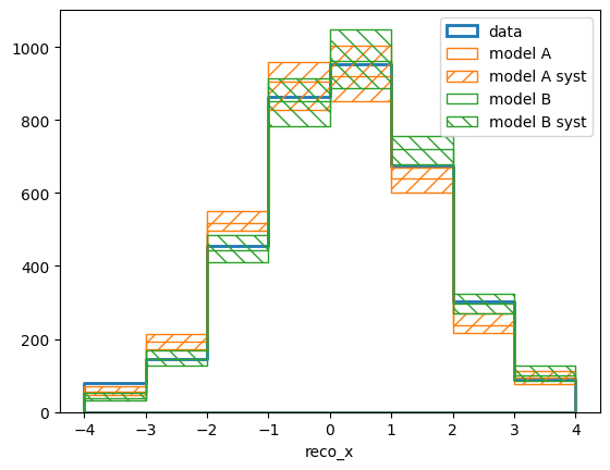
The modelX_syst_reco arrays now contain 100 different predictions, corresponding to the 100 detector variations. The parameter stac_function == 0.68 tells the plotter to draw the area of the central 68% of the range of predictions.

And of course we can compare the p-values of the two fitted models assuming the nominal detector response:

testA = likelihood.HypothesisTester(calcA)
testB = likelihood.HypothesisTester(calcB)
print(testA.max_likelihood_p_value())
print(testB.max_likelihood_p_value())

0.432
0.62

As well as the p-values yielded when taking the systematic uncertainties into account:

testA_syst = likelihood.HypothesisTester(calcA_syst)
testB_syst = likelihood.HypothesisTester(calcB_syst)
print(testA_syst.max_likelihood_p_value())
print(testB_syst.max_likelihood_p_value())

0.556
0.728

We can construct confidence intervals on the template weights of the models using the maximum likelihood p-value just like before:

p_values_A = []
p_values_B = []
p_values_A_syst = []
p_values_B_syst = []
values = np.linspace(600, 1600, 21)
for v in values:
    A = testA.max_likelihood_p_value([v])
    A_syst = testA_syst.max_likelihood_p_value([v])
    B = testB.max_likelihood_p_value([v])
    B_syst = testB_syst.max_likelihood_p_value([v])
    print(v, A, A_syst, B, B_syst)
    p_values_A.append(A)
    p_values_B.append(B)
    p_values_A_syst.append(A_syst)
    p_values_B_syst.append(B_syst)

fig, ax = plt.subplots()
ax.set_xlabel("Model weight")
ax.set_ylabel("p-value")
ax.plot(values, p_values_A, label="Model A", color='C1', linestyle='dotted')
ax.plot(values, p_values_A_syst, label="Model A syst", color='C1', linestyle='solid')
ax.plot(values, p_values_B, label="Model B", color='C2', linestyle='dotted')
ax.plot(values, p_values_B_syst, label="Model B syst", color='C2', linestyle='solid')
ax.axvline(retA.x[0], color='C1', linestyle='dotted')
ax.axvline(retA_syst.x[0], color='C1', linestyle='solid')
ax.axvline(retB.x[0], color='C2', linestyle='dotted')
ax.axvline(retB_syst.x[0], color='C2', linestyle='solid')
ax.axhline(0.32, color='k', linestyle='dashed')
ax.axhline(0.05, color='k', linestyle='dashed')
ax.legend(loc='best')
fig.savefig("p-values.png")

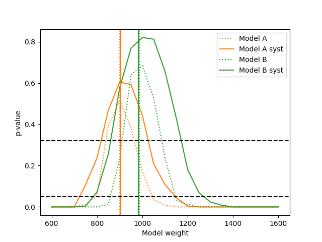
The “fixed” models have no free parameters here, making them degenerate. This means using the max_likelihood_p_value() is equivalent to testing the corresponding simple hypotheses using the likelihood_p_value(). No actual maximisation is taking place. Note that the p-values for model A are generally smaller than those for model B. This is consistent with previous results showing that the data is better described by model B.

Finally, let us construct confidence intervals of the template weights, assuming that the corresponding model is correct:

p_values_A = []
p_values_B = []
p_values_A_syst = []
p_values_B_syst = []
values = np.linspace(600, 1600, 21)
for v in values:
    A = testA.max_likelihood_ratio_p_value([v])
    A_syst = testA_syst.max_likelihood_ratio_p_value([v])
    B = testB.max_likelihood_ratio_p_value([v])
    B_syst = testB_syst.max_likelihood_ratio_p_value([v])
    print(v, A, A_syst, B, B_syst)
    p_values_A.append(A)
    p_values_B.append(B)
    p_values_A_syst.append(A_syst)
    p_values_B_syst.append(B_syst)

p_values_A_wilks = []
p_values_B_wilks = []
fine_values = np.linspace(600, 1600, 100)
for v in fine_values:
    A = testA_syst.wilks_max_likelihood_ratio_p_value([v])
    B = testB_syst.wilks_max_likelihood_ratio_p_value([v])
    print(v, A, B)
    p_values_A_wilks.append(A)
    p_values_B_wilks.append(B)

fig, ax = plt.subplots()
ax.set_xlabel("Model weight")
ax.set_ylabel("p-value")
ax.plot(values, p_values_A, label="Model A", color='C1', linestyle='dotted')
ax.plot(values, p_values_A_syst, label="Model A syst", color='C1', linestyle='solid')
ax.plot(fine_values, p_values_A_wilks, label="Model A Wilks", color='C1', linestyle='dashed')
ax.plot(values, p_values_B, label="Model B", color='C2', linestyle='dotted')
ax.plot(values, p_values_B_syst, label="Model B syst", color='C2', linestyle='solid')
ax.plot(fine_values, p_values_B_wilks, label="Model B Wilks", color='C2', linestyle='dashed')
ax.axvline(retA.x[0], color='C1', linestyle='dotted')
ax.axvline(retA_syst.x[0], color='C1', linestyle='solid')
ax.axvline(retB.x[0], color='C2', linestyle='dotted')
ax.axvline(retB_syst.x[0], color='C2', linestyle='solid')
ax.axhline(0.32, color='k', linestyle='dashed')
ax.axhline(0.05, color='k', linestyle='dashed')
ax.legend(loc='best')
fig.savefig("ratio-p-values.png")

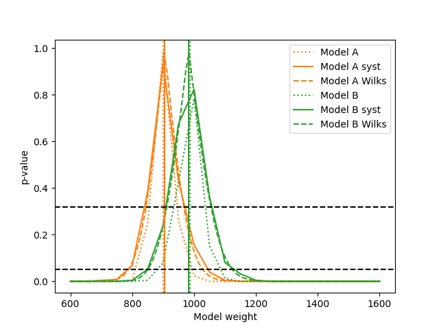
Note that the p-values for both models go up to 1.0 here (within the granularity of the parameter scan) and that the constructed confidence intervals are very different from the ones before. This is because we are asking a different question now. Before we asked the question “What is the probability of getting a worse likelihood assuming that the tested model-parameter is true?”. Now we ask the question “What is the probability of getting a worse best-fit likelihood ratio, assuming the tested model-parameter is true?”. Since the likelihood ratio is 1.0 at the best fit point and the likelihood ratio of nested hypotheses is less than or equal to 1.0 by construction, the p-value is 100% there.

The method wilks_max_likelihood_ratio_p_value() calculates the same p-value as max_likelihood_ratio_p_value(), but does so assuming Wilks’ theorem holds. This does not require the generation of random data and subsequent likelihood maximisations, so it is much faster.