Example 00 – Basic usage of binnings
Aims
Create “real” and simulated data of the mock experiemnt
Load data into histograms and plot it
Instructions
The folder ../simple_experiment/ contains two scripts to create “real” and
simulated data. The script ‘simulate_experiment.py’ simulates the mock
experiment and creates two files: one file with the truth information of all
simulated events, and another file with the truth and reconstructed information
of all reconstructed events. The command line parameters determine the
properties of the simulation, e.g. whether to simulate background or signal and
what signal model to use.
The script run_experiment.py creates a single file with only reconstructed
information. Of course, this file is also the result of simulations, but since
it is supposed to represent the real results of a real experiment, no truth
information is saved.
Create “real” data corresponding to ten years of running the experiment:
$ ../simple_experiment/run_experiment.py 10 real_data.txt
Create simulated data corresponding to ten times the real data:
$ ../simple_experiment/simulate_experiment.py 100 modelA modelA_data.txt modelA_truth.txt
$ ../simple_experiment/simulate_experiment.py 100 modelB modelB_data.txt modelB_truth.txt
The file reco-binning.yml contains a RectilinearBinning object
for the reconstructed information:
!RectilinearBinning
variables:
- reco_x
- reco_y
bin_edges:
- [-.inf,
  ...
  .inf]
- [-.inf,
  ...
  .inf]
include_upper: false
A RectilinearBinning object defines bin edges in multiple variables.
These variables are orthogonal to each other. The total number of bins is thus
the product of the number of bins per variable.
Let’s create a binning object, load the data into it, and plot the distributions:
from remu import binning
from remu import plotting
with open("reco-binning.yml", 'r') as f:
reco_binning = binning.yaml.full_load(f)
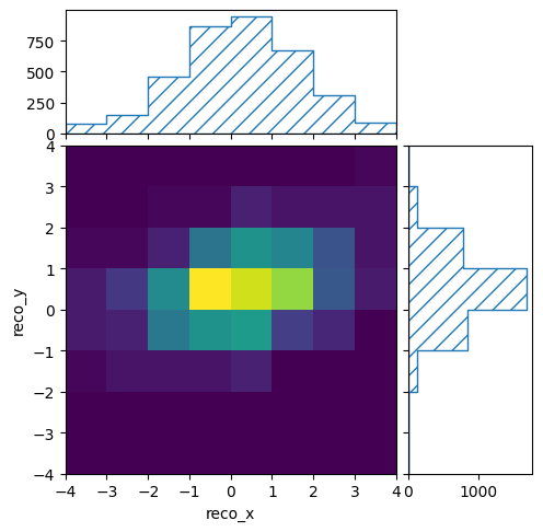
reco_binning.fill_from_csv_file("real_data.txt")
pltr = plotting.get_plotter(reco_binning)
pltr.plot_values()
pltr.savefig("real_data.png")
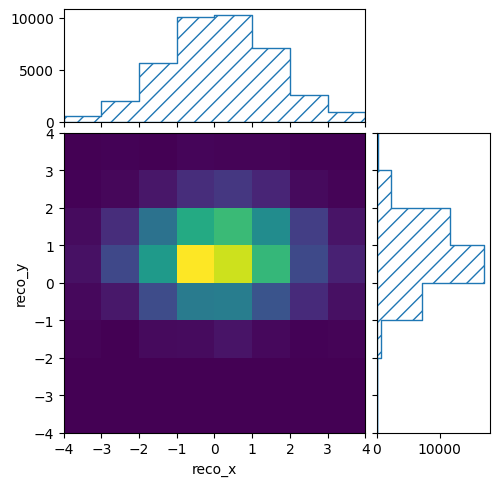
reco_binning.reset()
reco_binning.fill_from_csv_file("modelA_data.txt")

pltr = plotting.get_plotter(reco_binning)
pltr.plot_values()
pltr.savefig("modelA_data.png")
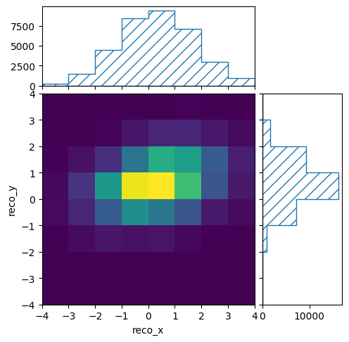
reco_binning.reset()
reco_binning.fill_from_csv_file("modelB_data.txt")

pltr = plotting.get_plotter(reco_binning)
pltr.plot_values()
pltr.savefig("modelB_data.png")
Plotting the different kinds of Binning objects is handled by their
respective BinningPlotter classes. The function
plotting.get_plotter() will return an instance of the appropriate
plotting class for the provided binning, in this case a
RectilinearBinningPlotter.
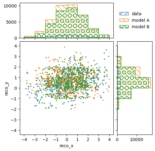
The RectilinearBinningPlotter supports the scatter parameter,
which makes it draw pseudo scatter plots instead of 2D histograms. This is
useful to compare multiple distributions in the same plot:
pltr = plotting.get_plotter(reco_binning)
reco_binning.reset()
reco_binning.fill_from_csv_file("real_data.txt")
pltr.plot_values(label="data", scatter=500)
reco_binning.reset()
reco_binning.fill_from_csv_file("modelA_data.txt")
pltr.plot_values(label="model A", scatter=500)
reco_binning.reset()
reco_binning.fill_from_csv_file("modelB_data.txt")
pltr.plot_values(label="model B", scatter=500)
pltr.legend()
pltr.savefig("compare_data.png")
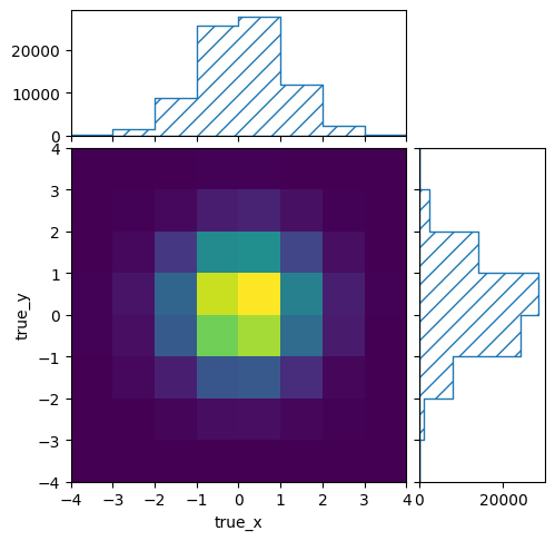
We can do the same with the true information and its respective binning in ‘truth-binning.yml’:
with open("truth-binning.yml", 'r') as f:
    truth_binning = binning.yaml.full_load(f)

truth_binning.fill_from_csv_file("modelA_truth.txt")

pltr = plotting.get_plotter(truth_binning)
pltr.plot_values()
pltr.savefig("modelA_truth.png")
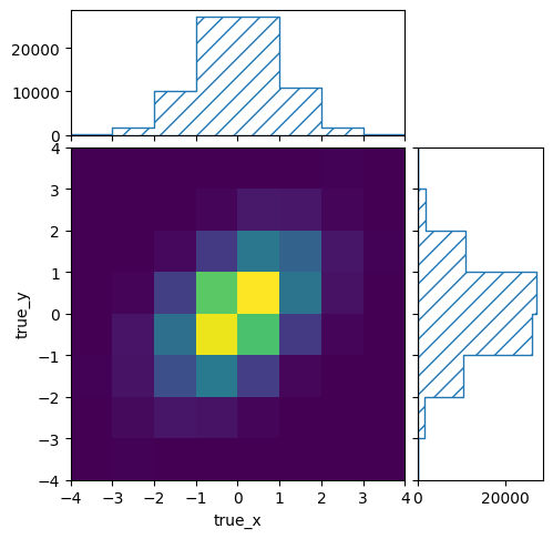
truth_binning.reset()
truth_binning.fill_from_csv_file("modelB_truth.txt")

pltr = plotting.get_plotter(truth_binning)
pltr.plot_values()
pltr.savefig("modelB_truth.png")
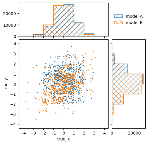
pltr = plotting.get_plotter(truth_binning)
truth_binning.reset()
truth_binning.fill_from_csv_file("modelA_truth.txt")
pltr.plot_values(label="model A", scatter=500)
truth_binning.reset()
truth_binning.fill_from_csv_file("modelB_truth.txt")
pltr.plot_values(label="model B", scatter=500)
pltr.legend()
pltr.savefig("compare_truth.png")