Example 02 – Simple model fits
Aims
Create a
LikelihoodCalculatorwith the response matrix and experiment dataCalculate likelihoods of model predictions
Create a
HypothesisTesterand calculate p-valuesFit parameters and calculate p-values of composite hypotheses
Construct confidence intervals of parameters of composite hypotheses
Instructions
The calculation of likelihoods and p-values is handled by the classes in the
likelihood module:
import numpy as np
from remu import binning
from remu import plotting
from remu import likelihood
Some calculations handled in this module can be parallelized by setting the
mapper function to something that uses parallel processes or threads, e.g.
the map function of a multiprocess.Pool object:
from multiprocess import Pool
pool = Pool(8)
likelihood.mapper = pool.map
This is completely optional, but can speed up the calculation of p-values
considerably. Please not the use of the multiprocess package, instead of
Python’s native multiprocessing. The latter does not support the pickling
of arbitrary functions, so it does not work.
First we will create DataModel and ResponseMatrixPredictor
objects from the information of the previous examples:
response_matrix = "../01/response_matrix.npz"

with open("../01/reco-binning.yml", 'rt') as f:
    reco_binning = binning.yaml.full_load(f)
with open("../01/optimised-truth-binning.yml", 'rt') as f:
    truth_binning = binning.yaml.full_load(f)

reco_binning.fill_from_csv_file("../00/real_data.txt")
data = reco_binning.get_entries_as_ndarray()
data_model = likelihood.PoissonData(data)
matrix_predictor = likelihood.ResponseMatrixPredictor(response_matrix)
The data model knows how to compare event rate predictions to the data and
calculate the respective likelihoods, in this case using Poisson statistics.
The matrix predictor contains the information of the previously built response
matrix and is used to predict reco-space event rates from truth-space event
rates. These two can now be combined into a LikelihoodCalculator and
HypothesisTester:
calc = likelihood.LikelihoodCalculator(data_model, matrix_predictor)
test = likelihood.HypothesisTester(calc)
Likelihood calculators are in charge of computing likelihoods of parameter sets. In this case, it will calculate the likelihoods of truth-space event-rates, as that is what the predictor is expecting as parameters. Hypothesis testers use the likelihood calculator to do statistical tests and calculate p-values.
Now we need some models to test against the data. We will use the models A and B of the previous steps, but we will turn them into area-normalised templates:
truth_binning.fill_from_csv_file("../00/modelA_truth.txt")
modelA = truth_binning.get_values_as_ndarray()
modelA /= np.sum(modelA)

truth_binning.reset()
truth_binning.fill_from_csv_file("../00/modelB_truth.txt")
modelB = truth_binning.get_values_as_ndarray()
modelB /= np.sum(modelB)
Let us calculate some likelihoods and p-values with these templates, assuming total of 1000 expected events in the truth space (i.e. before efficiency effects):
print(calc(modelA*1000))
print(test.likelihood_p_value(modelA*1000))
print(calc(modelB*1000))
print(test.likelihood_p_value(modelB*1000))
-27.800234247380704
0.1968
-24.480283069694824
0.6804
The exact results may vary due to statistical fluctuations. Especially the p-values are calculated by generating random data sets assuming the tested model is true. The fraction of data sets with a worse likelihood than the actual measured one is the p-value. Depending on the required confidence level, we could exclude the “1000*A” hypothesis, while the “1000*B” hypothesis is more compatible with the data.
Models that predict the true distribution of events usually have some free parameters. For example we could assume that the shapes of models A and B are well motivated but the total number of events is not well predicted. To test these more flexible models, we can create predictors that take the free parameters of the models as inputs and predict event rates in truth space. By composing (i.e. “chaining”) these predictors to the matrix predictor, we can then build a likelihood calculator that takes these parameters as inputs directly:
modelA_shape = likelihood.TemplatePredictor([modelA])
modelA_reco_shape = matrix_predictor.compose(modelA_shape)
calcA = likelihood.LikelihoodCalculator(data_model, modelA_reco_shape)
This example uses the TemplatePredictor class, which takes a list of
templates as its initialisation parameter and creates a predictor with one
template weight parameter per template. Since we only provide one template
here, it only takes one parameter.
We can now do a maximum likelihood fit with the model, using a
BasinHoppingMaximiser:
maxi = likelihood.BasinHoppingMaximizer()
retA = maxi(calcA)
print(retA)
                        fun: 25.257278617610154
             log_likelihood: -25.257278617610154
 lowest_optimization_result:       fun: 25.257278617610154
 hess_inv: <1x1 LbfgsInvHessProduct with dtype=float64>
      jac: array([6.75015063e-06])
  message: 'CONVERGENCE: NORM_OF_PROJECTED_GRADIENT_<=_PGTOL'
     nfev: 20
      nit: 4
     njev: 10
   status: 0
  success: True
        x: array([900.29272504])
                    message: ['requested number of basinhopping iterations completed successfully']
      minimization_failures: 0
                       nfev: 140
                        nit: 10
                       njev: 70
                    success: True
                          x: array([900.29272504])
The parameter values of the maximum likelihood solution are returned as
ret.x. The actual maximum log likelihood is stored in
ret.log_likelihood. The other properties of the returned object show the
status of the optimisation and are not important for this example.
Instead of composing the predictors and building a new likelihood calculator with the result, it is also possible to directly compose the model predictor with the likelihood calculator:
modelB_shape = likelihood.TemplatePredictor([modelB])
calcB = calc.compose(modelB_shape)
retB = maxi(calcB)
print(retB)
                        fun: 24.439068081734
             log_likelihood: -24.439068081734
 lowest_optimization_result:       fun: 24.439068081734
 hess_inv: <1x1 LbfgsInvHessProduct with dtype=float64>
      jac: array([7.10542172e-07])
  message: 'CONVERGENCE: NORM_OF_PROJECTED_GRADIENT_<=_PGTOL'
     nfev: 18
      nit: 4
     njev: 9
   status: 0
  success: True
        x: array([986.50497796])
                    message: ['requested number of basinhopping iterations completed successfully']
      minimization_failures: 0
                       nfev: 104
                        nit: 10
                       njev: 52
                    success: True
                          x: array([986.50497796])
The maximum likelihood solutions for model A shows a lower number of events
than that of model B. This is due to the higher average efficiency of
reconstructing the events of model A, i.e. their distribution in y. The
maximum log likelihood of model B is higher than for model A. So model B is
able to describe the given data better than model A. This is also reflected in
the p-values:
testA = likelihood.HypothesisTester(calcA, maximizer=maxi)
testB = likelihood.HypothesisTester(calcB, maximizer=maxi)
print(testA.max_likelihood_p_value())
print(testB.max_likelihood_p_value())
0.428
0.54
Here we explicitly told the hypothesis testers which maximiser to use, but this is optional.
Again the p-value is calculated from randomly generated data sets assuming the given model is true. This time it is the ratio of data sets that yield a worse maximum likelihood though. This means a fit is performed for each mock data set.
We can also take a qualitative look at the fit of data and the two models by plotting the result in reco space:
pltr = plotting.get_plotter(reco_binning)
pltr.plot_entries(label='data', hatch=None)
modelA_reco, modelA_weights = modelA_reco_shape(retA.x)
modelA_logL = calcA(retA.x)
modelA_p = testA.likelihood_p_value(retA.x)
modelB_reco, modelB_weights = calcB.predictor(retB.x)
modelB_logL = calcB(retB.x)
modelB_p = testB.likelihood_p_value(retB.x)
pltr.plot_array(modelA_reco,
    label='model A: $\log L=%.1f$, $p=%.3f$'%(modelA_logL, modelA_p),
    hatch=None, linestyle='dashed')
pltr.plot_array(modelB_reco,
    label='model B: $\log L=%.1f$, $p=%.3f$'%(modelB_logL, modelB_p),
    hatch=None, linestyle='dotted')
pltr.legend(loc='lower center')
pltr.savefig("reco-comparison.png")
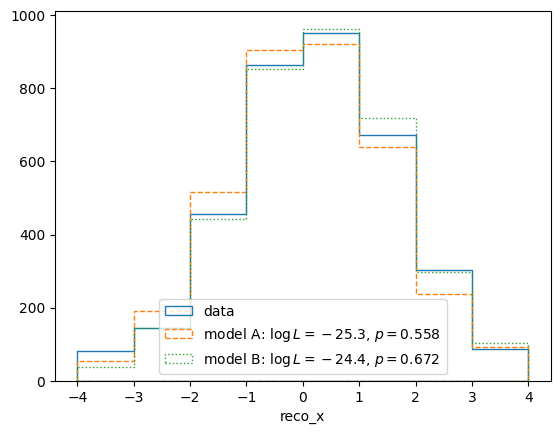
The p-value shown in this plot is again the likelihood_p_value() (as
opposed to the max_likelihood_p_value()). This is a better
representation of the goodness of fit of the maximum likelihood solution,
roughly equivalent to checking for a “chi-square” close to the number of bins.
The return values of the predictors are formated to accomodate multiple weighted predictions per set of parameters, i.e. systematic incertainties. We can ignore the weights for now.
Usually there is more than one template to be fitted to the data. Let’s see what happens if we allow combinations of model A and B:
mix_model = likelihood.TemplatePredictor([modelA, modelB])
calc_mix = calc.compose(mix_model)
ret = maxi.maximize_log_likelihood(calc_mix)
print(ret)
                        fun: 23.818800345296474
             log_likelihood: -23.818800345296474
 lowest_optimization_result:       fun: 23.818800345296474
 hess_inv: <2x2 LbfgsInvHessProduct with dtype=float64>
      jac: array([0.00000000e+00, 2.84216869e-06])
  message: 'CONVERGENCE: NORM_OF_PROJECTED_GRADIENT_<=_PGTOL'
     nfev: 87
      nit: 4
     njev: 29
   status: 0
  success: True
        x: array([351.46741373, 601.38025556])
                    message: ['requested number of basinhopping iterations completed successfully']
      minimization_failures: 0
                       nfev: 273
                        nit: 10
                       njev: 91
                    success: True
                          x: array([351.46741373, 601.38025556])
test = likelihood.HypothesisTester(calc_mix)
print(test.max_likelihood_p_value())
0.664
The two parameters of this new combined model are the weights of model A and B respectively. This allows a contribution of model A in the maximum likelihood solution.
It might be useful to calculate a confidence interval for a parameter embedded in a larger hypothesis with more parameters. This can be done by fixing that parameter at different values (reducing the number of free parameters) and calculating the likelihood ratio of this new embedded hypothesis and the embedding original hypothesis. Comparing this likelihood ratio with the expected distribution of likelihood ratios assuming the embedded hypothesis is true yields p-values that can be used to construct the confidence interval:
p_values = []
A_values = np.linspace(0, 1000, 11)
for A in A_values:
    p = test.max_likelihood_ratio_p_value((A,None))
    print(A, p)
    p_values.append(p)
Calculating these might take a while. The method
max_likelihood_ratio_p_value() fixes the specified parameters and
generates toy data sets at the best fit point of the remaining parameters. It
then computes the maximum likelihoods for both the fixed and unfixed version of
the predictors for all toy data sets. The fraction of toy data sets with an
equal or worse maximum likelihood ratio then the real data is the p-value.
This p-value is sometimes called the “profile plug-in p-value”, as one “plugs in” the maximum likelihood estimate of the hypothesis’ (nuisance) parameters to generate the toy data and calculate the p-value. It’s coverage properties are not exact, so care has to be taken to make sure it performs as expected (e.g. by testing it with simulated data).
In the limit of “large statistics”, the maximum log likelihood ratio should be distributed like a chi-square distribution, according to Wilks’ theorem. This can be used to speed up the calculation of p-values considerably, as it skips the generation of fit to toy data sets:
wilks_p_values = []
fine_A_values = np.linspace(0, 1000, 100)
for A in fine_A_values:
    p = test.wilks_max_likelihood_ratio_p_value((A,None))
    print(A, p)
    wilks_p_values.append(p)
This can then be plotted with your usual plotting libraries:
from matplotlib import pyplot as plt
fig, ax = plt.subplots()
ax.set_xlabel("Model A weight")
ax.set_ylabel("p-value")
ax.plot(A_values, p_values, label="Profile plug-in")
ax.plot(fine_A_values, wilks_p_values, label="Wilks")
ax.axvline(ret.x[0], color='k', linestyle='solid')
ax.axhline(0.32, color='k', linestyle='dashed')
ax.axhline(0.05, color='k', linestyle='dashed')
ax.legend(loc='best')
fig.savefig("p-values.png")
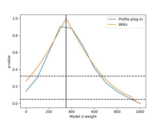
The confidence interval is the region of the parameter space with a p-value over the desired test significance. The maximum likelihood solution is shown as vertical line. Please note that this assumes that the full hypothesis with no fixed parameters is true, i.e. that some combination of model A and model B templates actually describes reality.