Example 04 – Markov Chain Monte Carlo

Aims

• Use LikelihoodCalculator objects in a Marcov Chain Monte Carlo Sampling

Instructions

LikelihoodCalculator objects allow direct access to the likelihood function of theoretical models given the measured data. As such they can easily be used in Bayesian inference using Marcov Chain Monte Carlo (MCMC) methods.

ReMU has some built-in support to simplyfy the use of LikelihoodCalculator objects with emcee, a MCMC package for python:

https://emcee.readthedocs.io/

Before we can use the MCMC, we have to create the response matrix, LikelihoodCalculator objects, just like in the previous examples:

import numpy as np
from matplotlib import pyplot as plt
from remu import binning
from remu import plotting
from remu import likelihood
from remu import likelihood_utils
import emcee

with open("../01/reco-binning.yml", 'rt') as f:
    reco_binning = binning.yaml.full_load(f)
with open("../01/optimised-truth-binning.yml", 'rt') as f:
    truth_binning = binning.yaml.full_load(f)

reco_binning.fill_from_csv_file("../00/real_data.txt")
data = reco_binning.get_entries_as_ndarray()
data_model = likelihood.PoissonData(data)

response_matrix = "../03/response_matrix.npz"
matrix_predictor = likelihood.ResponseMatrixPredictor(response_matrix)
calc = likelihood.LikelihoodCalculator(data_model, matrix_predictor)

truth_binning.fill_from_csv_file("../00/modelA_truth.txt")
modelA = truth_binning.get_values_as_ndarray()
modelA /= np.sum(modelA)

modelA_shape = likelihood.TemplatePredictor([modelA])
calcA = calc.compose(modelA_shape)

Now we can create a sampler and inital guesses for the parameters using the likelihood_utils module:

samplerA = likelihood_utils.emcee_sampler(calcA)
guessA = likelihood_utils.emcee_initial_guess(calcA)

These can then be used to draw from the posterior distribution. Since the likelihood function used here is not modified by a prior, this is equivalent to using flat priors for the parameters. See the emcee documentation for details about how to use these objects:

state = samplerA.run_mcmc(guessA, 100)
chain = samplerA.get_chain(flat=True)
print(chain.shape)

(200, 1)

Note that the number of data points is higher than the requested chain length. This is due to the fact that emcee will sample multiple chains in parallel, which get combined into one long chain when using the flat option. The number of chains depends on the number of free parameters.

We can now plot the distribution of the template weight parameter:

fig, ax = plt.subplots()
ax.hist(chain[:,0])
ax.set_xlabel("model A weight")
fig.savefig("burn_short.png")

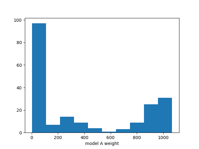
There clearly is something wrong with this distribution. The MCMC has not converged yet. The authors of emcee suggest to use the autocorrelation time as a measure of whether a chain has converged:

try:
    tau = samplerA.get_autocorr_time()
    print(tau)
except emcee.autocorr.AutocorrError as e:
    print(e)

The chain is shorter than 50 times the integrated autocorrelation time for 1 parameter(s). Use this estimate with caution and run a longer chain!
N/50 = 2;
tau: [13.27761416]

So let us try again with a longer chain:

samplerA.reset()
state = samplerA.run_mcmc(guessA, 200*50)
chain = samplerA.get_chain(flat=True)

try:
    tau = samplerA.get_autocorr_time()
    print(tau)
except emcee.autocorr.AutocorrError as e:
    print(e)

[47.5875875]

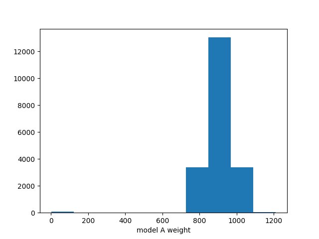
Now the chain is long enough and we can have another look at the distribution:

fig, ax = plt.subplots()
ax.hist(chain[:,0])
ax.set_xlabel("model A weight")
fig.savefig("burn_long.png")

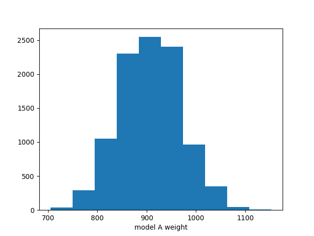
Now we can discard these events and generate a new set from the last state of the sampler:

samplerA.reset()
state = samplerA.run_mcmc(state, 100*50)
chain = samplerA.get_chain(flat=True)

try:
    tau = samplerA.get_autocorr_time()
    print(tau)
except emcee.autocorr.AutocorrError as e:
    print(e)

[27.64249535]

fig, ax = plt.subplots()
ax.hist(chain[:,0])
ax.set_xlabel("model A weight")
fig.savefig("weightA.png")

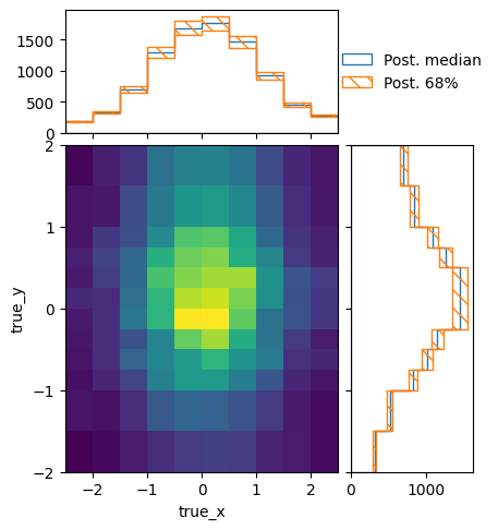
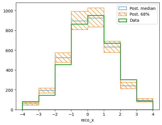
We can also take a look at how these predictions look in truth and reco space:

truth, _ = modelA_shape(chain)
truth.shape = (np.prod(truth.shape[:-1]), truth.shape[-1])
pltr = plotting.get_plotter(truth_binning)
pltr.plot_array(truth, stack_function=np.median, label="Post. median", hatch=None)
pltr.plot_array(truth, stack_function=0.68, label="Post. 68%", scatter=0)
pltr.legend()
pltr.savefig("truthA.png")

reco, _ = calcA.predictor(chain)
reco.shape = (np.prod(reco.shape[:-1]), reco.shape[-1])
pltr = plotting.get_plotter(reco_binning)
pltr.plot_array(reco, stack_function=np.median, label="Post. median", hatch=None)
pltr.plot_array(reco, stack_function=0.68, label="Post. 68%")
pltr.plot_array(data, label="Data", hatch=None, linewidth=2)
pltr.legend()
pltr.savefig("recoA.png")

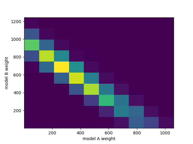
All of this also works with more parameters, of course:

truth_binning.reset()
truth_binning.fill_from_csv_file("../00/modelB_truth.txt")
modelB = truth_binning.get_values_as_ndarray()
modelB /= np.sum(modelB)

combined = likelihood.TemplatePredictor([modelA, modelB])
calcC = calc.compose(combined)

samplerC = likelihood_utils.emcee_sampler(calcC)
guessC = likelihood_utils.emcee_initial_guess(calcC)

state = samplerC.run_mcmc(guessC, 200*50)
chain = samplerC.get_chain(flat=True)
print(chain.shape)

(40000, 2)

try:
    tau = samplerC.get_autocorr_time()
    print(tau)
except emcee.autocorr.AutocorrError as e:
    print(e)

[68.8796533  56.78473315]

samplerC.reset()
state = samplerC.run_mcmc(state, 100*50)
chain = samplerC.get_chain(flat=True)
try:
    tau = samplerC.get_autocorr_time()
    print(tau)
except emcee.autocorr.AutocorrError as e:
    print(e)

[84.59675341 99.31384933]

fig, ax = plt.subplots()
ax.hist2d(chain[:,0], chain[:,1])
ax.set_xlabel("model A weight")
ax.set_ylabel("model B weight")
fig.savefig("combined.png")

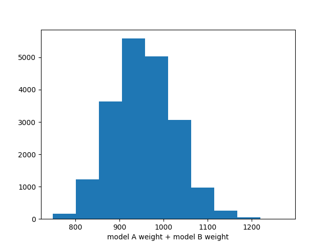
fig, ax = plt.subplots()
ax.hist(np.sum(chain, axis=-1))
ax.set_xlabel("model A weight + model B weight")
fig.savefig("total.png")