Example 05 – Backgrounds
Aims
Understand and deal with background events in measurements
Instructions
Real experiments will almost always include some sort of background or noise events in the recorded data. ReMU is well equipped to deal with those in a consistent fashion.
Let us first create the noisy data as well as simulations of background and noise events:
# Create "real" data
../simple_experiment/run_experiment.py 10 real_data.txt --enable-background

# Create BG simulation
../simple_experiment/simulate_experiment.py 100 background nominal_bg_data.txt bg_truth.txt

# Create Noise simulation
../simple_experiment/simulate_experiment.py 100 noise noise_data.txt noise_truth.txt

# Create Variations
../simple_experiment/vary_detector.py nominal_bg_data.txt bg_data.txt
In this context, we call “noise” events that are recorded, but that do not have a meaningful true information associated with them. “Background” on the other hand can be understood as regular events in the detector, but which we are not interested in (e.g. because they are created by a different process than our main subject of study).
Background events can behave differently than signal events, but because they also have a defined true information, we can treat them just like signal. The only difference is that they will occupy different truth bins than the signal events.
Noise events on the other hand do not have meaningful true properties, so we will just assign them all to a single truth bin. The content of that single bin will then determine the number of expected noise events in the reconstructed binnings.
Starting from the truth binning we created for the signal models in a previous example, let us create a binning for the background events:
import numpy as np
from remu import binning
from remu import migration
from remu import matrix_utils
from remu import plotting

builder = migration.ResponseMatrixArrayBuilder(1)

with open("../01/reco-binning.yml", 'rt') as f:
    reco_binning = binning.yaml.full_load(f)
with open("../01/optimised-truth-binning.yml", 'rt') as f:
    signal_binning = binning.yaml.full_load(f)

bg_binning = signal_binning.clone()
resp = migration.ResponseMatrix(reco_binning, bg_binning)
i = 0
resp.fill_from_csv_file("bg_data.txt", weightfield='weight_%i'%(i,),
    rename={'reco_x_%i'%(i,): 'reco_x'}, buffer_csv_files=True)
resp.fill_up_truth_from_csv_file("bg_truth.txt", buffer_csv_files=True)
entries = resp.get_truth_entries_as_ndarray()
while np.min(entries) < 10:
    resp = matrix_utils.improve_stats(resp)
    entries = resp.get_truth_entries_as_ndarray()
bg_binning = resp.truth_binning
bg_binning.reset()
reco_binning.reset()
This bg_binning will now include at least 10 events in each truth bin, when
building the response matrix.
Next we will create a binning that can distinguish between noise, background
and signal events, according to a variable aptly called event_type:
truth_binning = binning.LinearBinning(
    variable = 'event_type',
    bin_edges = [-1.5, -0.5, 0.5, 1.5],
    subbinnings = {
        1: bg_binning,
        2: signal_binning,
        }
    )

with open("truth-binning.yml", 'wt') as f:
    binning.yaml.dump(truth_binning, f)
The LinearBinning would have only three bins, but we insert the
previously created background and signal binnings as subbinnings into the
second and third bin respectively. This means that events which would fall into
those bins will get further subdivided by the subbinnings. We thus have a
binning that puts noise events (event_type == -1) into a single bin, sorts
background events (event_type == 0) according to bg_binning, and sorts
signal events (event_type == 1) according to signal_binning.
Now we create a ResponseMatrix with this binning, just like we did in
previous examples:
resp = migration.ResponseMatrix(reco_binning, truth_binning,
                                nuisance_indices=[0])
To fill the matrix, we need to tell it which event_type each event is,
though. This information might already be part of the simulated data, but
in this case we have to add that variable by hand.
For this we can use the cut_function parameter. A cut function takes the
data (a structured numpy array) as its only argument and returns the data that
should be filled into the binning:
import numpy.lib.recfunctions as rfn
def set_signal(data):
    return rfn.append_fields(data, 'event_type', np.full_like(data['true_x'], 1.))
def set_bg(data):
    return rfn.append_fields(data, 'event_type', np.full_like(data['true_x'], 0.))
def set_noise(data):
    return rfn.append_fields(data, 'event_type', np.full_like(data['reco_x'], -1.))

n_toys = 100
for i in range(n_toys):
    resp.reset()
    resp.fill_from_csv_file(["../03/modelA_data.txt", "../03/modelB_data.txt"],
        weightfield='weight_%i'%(i,), rename={'reco_x_%i'%(i,): 'reco_x'},
        cut_function=set_signal, buffer_csv_files=True)
    resp.fill_up_truth_from_csv_file(
        ["../00/modelA_truth.txt", "../00/modelB_truth.txt"],
        cut_function=set_signal, buffer_csv_files=True)
    resp.fill_from_csv_file("bg_data.txt", weightfield='weight_%i'%(i,),
        rename={'reco_x_%i'%(i,): 'reco_x'}, cut_function=set_bg,
        buffer_csv_files=True)
    resp.fill_up_truth_from_csv_file("bg_truth.txt", cut_function=set_bg,
        buffer_csv_files=True)
    # Calling `fill_up_truth_from_csv` twice only works because
    # the files fill completely different bins
    resp.fill_from_csv_file("noise_data.txt", cut_function=set_noise,
        buffer_csv_files=True)
    builder.add_matrix(resp)

builder.export("response_matrix.npz")
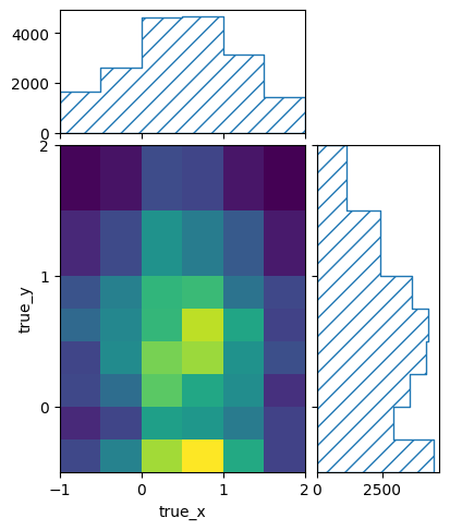
We can take a look at the truth information that has been filled into the last of the matrices:
pltr = plotting.get_plotter(truth_binning)
pltr.plot_values(density=False)
pltr.savefig('truth.png')
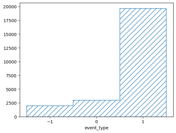
The base binning is a LinearBinning with only three bins. The
corresponding plotter does not know how to plot the subbinnings, so it just
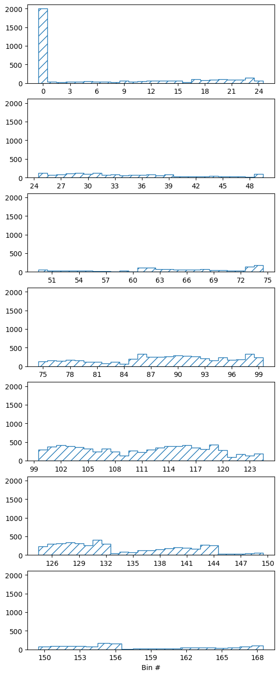
marginalizes them out. To plot the content of all truth bins, we can use the
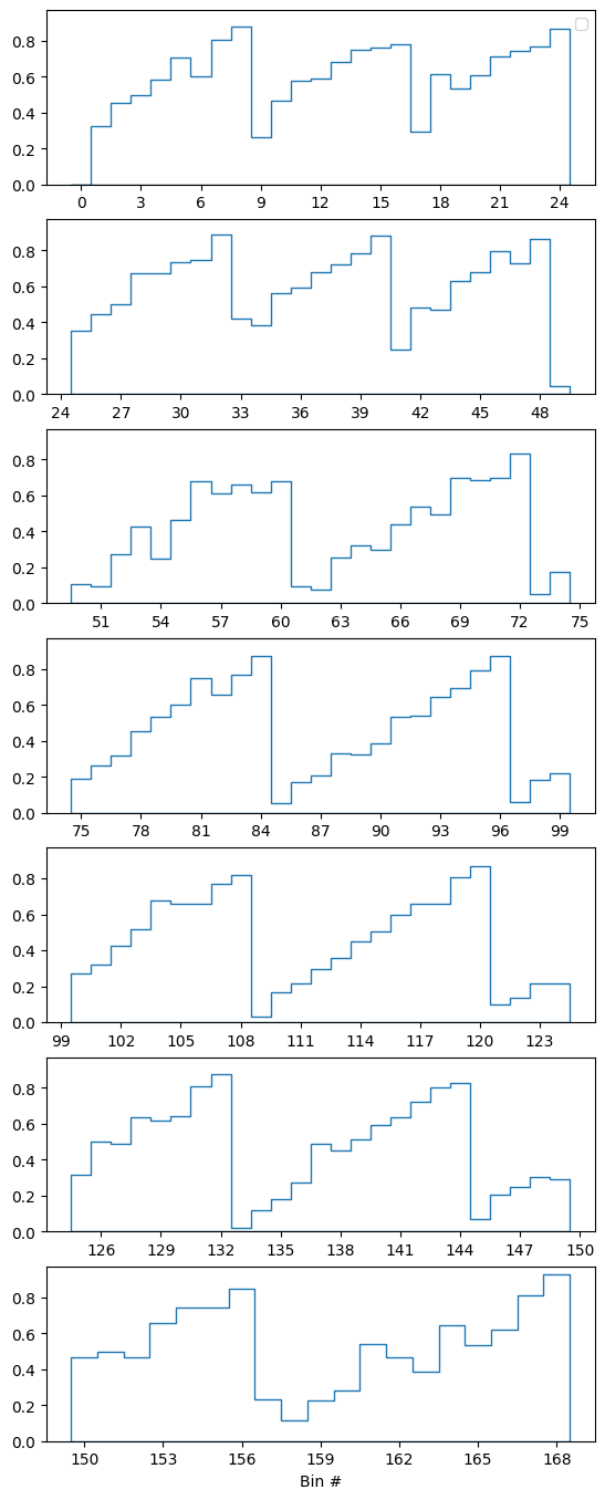
basic BinningPlotter, which simply plots the content of each bin:
pltr = plotting.BinningPlotter(truth_binning)
pltr.plot_values(density=False)
pltr.savefig('all_truth.png')
We can look at the content of the subbinings directly for some nicer plots:
pltr = plotting.get_plotter(signal_binning)
pltr.plot_values()
pltr.savefig('signal_truth.png')
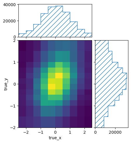
pltr = plotting.get_plotter(bg_binning)
pltr.plot_values()
pltr.savefig('bg_truth.png')
And we can take a look at the efficiencies using the corresponding convenience function:
matrix_utils.plot_mean_efficiency(resp, "efficiency.png")
Next we can use the response matrix for some hypothesis tests. First we need to
create the ResponseMatrixPredictor and the templates to be used with
the TemplatePredictor:
from remu import likelihood
from multiprocess import Pool
pool = Pool(8)
likelihood.mapper = pool.map

with open("../01/reco-binning.yml", 'rt') as f:
    reco_binning = binning.yaml.full_load(f)
with open("truth-binning.yml", 'rt') as f:
    truth_binning = binning.yaml.full_load(f)

reco_binning.fill_from_csv_file("real_data.txt")
data = reco_binning.get_entries_as_ndarray()
data_model = likelihood.PoissonData(data)

response_matrix = "response_matrix.npz"
matrix_predictor = likelihood.ResponseMatrixPredictor(response_matrix)

calc = likelihood.LikelihoodCalculator(data_model, matrix_predictor)
maxi = likelihood.BasinHoppingMaximizer()

import numpy.lib.recfunctions as rfn
def set_signal(data):
    return rfn.append_fields(data, 'event_type', np.full_like(data['true_x'], 1.))
def set_bg(data):
    return rfn.append_fields(data, 'event_type', np.full_like(data['true_x'], 0.))

truth_binning.fill_from_csv_file("../00/modelA_truth.txt",
                                 cut_function=set_signal)
modelA = truth_binning.get_values_as_ndarray()
modelA /= np.sum(modelA)

truth_binning.reset()
truth_binning.fill_from_csv_file("../00/modelB_truth.txt",
                                 cut_function=set_signal)
modelB = truth_binning.get_values_as_ndarray()
modelB /= np.sum(modelB)

truth_binning.reset()
truth_binning.fill_from_csv_file("bg_truth.txt", cut_function=set_bg)
bg = truth_binning.get_values_as_ndarray()
bg /= np.sum(bg)

truth_binning.reset()
noise = truth_binning.get_values_as_ndarray()
noise[0] = 1.
Since we put all noise events into the first truth bin, the noise template is just a value of 1 in that bin.
Now we start by trying to fit the model A template without background or noise events:
modelA_only = likelihood.TemplatePredictor([modelA])
calcA_only = calc.compose(modelA_only)

retA_only = maxi(calcA_only)
print(retA_only)
                        fun: 38.52930140475345
             log_likelihood: -38.52930140475345
 lowest_optimization_result:       fun: 38.52930140475345
 hess_inv: <1x1 LbfgsInvHessProduct with dtype=float64>
      jac: array([4.2633015e-06])
  message: 'CONVERGENCE: NORM_OF_PROJECTED_GRADIENT_<=_PGTOL'
     nfev: 54
      nit: 24
     njev: 27
   status: 0
  success: True
        x: array([1682.32663089])
                    message: ['requested number of basinhopping iterations completed successfully']
      minimization_failures: 0
                       nfev: 92
                        nit: 10
                       njev: 46
                    success: True
                          x: array([1682.32663089])
To judge how well the result actually fit, we can consult the results p-value:
testA_only = likelihood.HypothesisTester(calcA_only)
print(testA_only.likelihood_p_value(retA_only.x))
0.0024
It clearly is a very bad fit, which is reflected in the maximum likelihood p-value as well:
print(testA_only.max_likelihood_p_value())
0.0
So the signal-only model A hypothesis can be excluded. Now let us try again with background and noise templates added in:
modelA_bg = likelihood.TemplatePredictor([noise, bg, modelA])
calcA_bg = calc.compose(modelA_bg)

retA_bg = maxi(calcA_bg)
print(retA_bg)
                        fun: 28.30046763136394
             log_likelihood: -28.30046763136394
 lowest_optimization_result:       fun: 28.30046763136394
 hess_inv: <3x3 LbfgsInvHessProduct with dtype=float64>
      jac: array([-3.90798750e-06, -5.68433738e-06, -3.19743977e-06])
  message: 'CONVERGENCE: NORM_OF_PROJECTED_GRADIENT_<=_PGTOL'
     nfev: 124
      nit: 30
     njev: 31
   status: 0
  success: True
        x: array([ 99.5327942 , 476.05489184, 791.38644159])
                    message: ['requested number of basinhopping iterations completed successfully']
      minimization_failures: 0
                       nfev: 264
                        nit: 10
                       njev: 66
                    success: True
                          x: array([ 99.5327942 , 476.05489184, 791.38644159])
testA_bg = likelihood.HypothesisTester(calcA_bg)
print(testA_bg.likelihood_p_value(retA_bg.x))
0.9012
print(testA_bg.max_likelihood_p_value(), file=f)
0.62
This fit is clearly much better. We can repeat the same with model B:
modelB_only = likelihood.TemplatePredictor([modelB])
calcB_only = calc.compose(modelB_only)

retB_only = maxi(calcB_only)
print(retB_only)
                        fun: 37.51360728486539
             log_likelihood: -37.51360728486539
 lowest_optimization_result:       fun: 37.51360728486539
 hess_inv: <1x1 LbfgsInvHessProduct with dtype=float64>
      jac: array([-4.2633015e-06])
  message: 'CONVERGENCE: NORM_OF_PROJECTED_GRADIENT_<=_PGTOL'
     nfev: 78
      nit: 22
     njev: 39
   status: 0
  success: True
        x: array([1866.10415724])
                    message: ['requested number of basinhopping iterations completed successfully']
      minimization_failures: 0
                       nfev: 124
                        nit: 10
                       njev: 62
                    success: True
                          x: array([1866.10415724])
testB_only = likelihood.HypothesisTester(calcB_only)
print(testB_only.likelihood_p_value(retB_only.x))
0.002
print(testB_only.max_likelihood_p_value())
0.004
modelB_bg = likelihood.TemplatePredictor([noise, bg, modelB])
calcB_bg = calc.compose(modelB_bg)

retB_bg = maxi(calcB_bg)
print(retB_bg)
                        fun: 27.239578250837532
             log_likelihood: -27.239578250837532
 lowest_optimization_result:       fun: 27.239578250837532
 hess_inv: <3x3 LbfgsInvHessProduct with dtype=float64>
      jac: array([7.10542172e-06, 1.42108434e-06, 2.13165075e-06])
  message: 'CONVERGENCE: NORM_OF_PROJECTED_GRADIENT_<=_PGTOL'
     nfev: 48
      nit: 7
     njev: 12
   status: 0
  success: True
        x: array([ 210.20797605,  188.07865899, 1044.45892048])
                    message: ['requested number of basinhopping iterations completed successfully']
      minimization_failures: 0
                       nfev: 336
                        nit: 10
                       njev: 84
                    success: True
                          x: array([ 210.20797605,  188.07865899, 1044.45892048])
testB_bg = likelihood.HypothesisTester(calcB_bg)
print(testB_bg.likelihood_p_value(retB_bg.x))
0.98
print(testB_bg.max_likelihood_p_value())
0.796
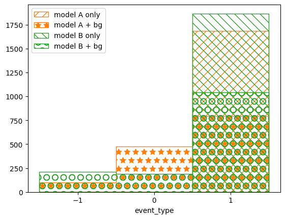
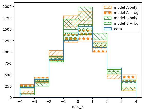
We can also take a qualitative look at the results by plotting the maximum likelihood predictions in reco and truth space:
pltr = plotting.get_plotter(reco_binning)
modelA_reco, modelA_weights = calcA_only.predictor(retA_only.x)
modelB_reco, modelB_weights = calcB_only.predictor(retB_only.x)
modelA_bg_reco, modelA_bg_weights = calcA_bg.predictor(retA_bg.x)
modelB_bg_reco, modelB_bg_weights = calcB_bg.predictor(retB_bg.x)
pltr.plot_array(modelA_reco, label='model A only', stack_function=0.68,
                hatch=r'//', edgecolor='C1')
pltr.plot_array(modelA_bg_reco, label='model A + bg', stack_function=0.68,
                hatch=r'*', edgecolor='C1')
pltr.plot_array(modelB_reco, label='model B only', stack_function=0.68,
                hatch=r'\\', edgecolor='C2')
pltr.plot_array(modelB_bg_reco, label='model B + bg', stack_function=0.68,
                hatch=r'O', edgecolor='C2')
pltr.plot_entries(edgecolor='C0', label='data', hatch=None, linewidth=2.)
pltr.legend()
pltr.savefig('reco-comparison.png')
pltr = plotting.get_plotter(truth_binning)
pltr.plot_array(modelA_only(retA_only.x)[0], label='model A only',
                hatch=r'//', edgecolor='C1', density=False)
pltr.plot_array(modelA_bg(retA_bg.x)[0], label='model A + bg',
                hatch=r'*', edgecolor='C1', density=False)
pltr.plot_array(modelB_only(retB_only.x)[0], label='model B only',
                hatch=r'\\', edgecolor='C2', density=False)
pltr.plot_array(modelB_bg(retB_bg.x)[0], label='model B + bg',
                hatch=r'O', edgecolor='C2', density=False)
pltr.legend(loc='upper left')
pltr.savefig('truth-comparison.png')