Example 04 – Markov Chain Monte Carlo
Aims
- Use
mcmc()to create a PyMC MCMC object - Use Markov Chain Monte Carlo to create a posterior sample of
CompositeHypothesisparameters - Compare two hypotheses using
marginal_log_likelihood()to calculate the Bayes factor - Compare two hypotheses using
plr()to calculate the Posterior Distribution of the Likelihood Ratio - Use a
JeffreysPrior
Instructions
ReMU has built-in support for generating Markov Chain Monte Carlo (MCMC) samples using the PyMC package. This example will only give a basic example of how to use this package in conjunction with ReMU. For detailed description of PyMC’s functionality, please refer to its documentation:
https://pymcmc.readthedocs.io/en/latest/
Before we can use the MCMC, we have to create the response matrix,
LikelihoodMachine, just like in the previous examples:
from six import print_
import numpy as np
from matplotlib import pyplot as plt
from remu import binning
from remu import likelihood
import pymc

with open("../01/reco-binning.yml", 'rt') as f:
    reco_binning = binning.yaml.load(f)
with open("../01/optimised-truth-binning.yml", 'rt') as f:
    truth_binning = binning.yaml.load(f)

reco_binning.fill_from_csv_file("../00/real_data.txt")
data = reco_binning.get_entries_as_ndarray()

response_matrix = "../03/response_matrix.npz"
lm = likelihood.LikelihoodMachine(data, response_matrix, limit_method='prohibit')
Because the MCMC is a Bayesian method, we need to define prior probabilities
for the parameters of the CompositeHypothesis we want to test.
Explaining how to choose an “objective” prior (or defining what that even is),
is out of scope of this example. Let us just use a simple flat prior for the
template weights. Because we already know that the total number of events is
somewhere around 1000, we will constrain the prior to the interval (0, 2000):
truth_binning.fill_from_csv_file("../00/modelA_truth.txt")
modelA = truth_binning.get_values_as_ndarray()
modelA /= np.sum(modelA)
truth_binning.reset()
truth_binning.fill_from_csv_file("../00/modelB_truth.txt")
modelB = truth_binning.get_values_as_ndarray()
modelB /= np.sum(modelB)

def flat_prior(value=100):
    if value >= 0 and value <= 2000:
        return 0
    else:
        return -np.inf

modelA_shape = likelihood.TemplateHypothesis([modelA], parameter_priors=[flat_prior],
    parameter_names=["template_weight"])
modelB_shape = likelihood.TemplateHypothesis([modelB], parameter_priors=[flat_prior],
    parameter_names=["template_weight"])
The function defining the prior must take one keyword argument value and
return the log of the prior probability. It must define a default value for
value, which must lie inside the allowed region of the parameter space. It
is used as the starting point for the MCMC evaluation. Since we are creating
TemplateHypothesis with only one template each, the parameter is only
a single floating point number: the template weight. If we used multiple
templates, the parameter would be a 1D array with all template weights.
With these CompositeHypothesis we can now create a MCMC
object and sample the posterior distribution of the parameter (see PyMC
documentation):
mcmcA = lm.mcmc(modelA_shape)

mcmcA.sample(iter=1000)
pymc.Matplot.plot(mcmcA, suffix='_noburn')
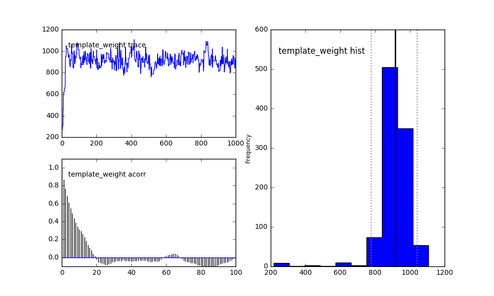
One can clearly see the effect of starting point in the top left trace of the
sample. Depending on how long it takes the MCMC to converge to the true
posterior distribution, this kind of effect can seriously bias your results. To
remove the biased part from the trace, we can use the burn argument. It
tells the sampler to just throw away the specified number of samples at the
beginning of the trace:
mcmcA.sample(iter=1000, burn=100)
pymc.Matplot.plot(mcmcA, suffix='_burn')

The bottom left plot still shows a considerable auto-correlation in the trace,
meaning it is not a true random sample of the posterior distribution. This can
be “fixed” with the thin argument. It tells the sampler to only store every
Nth sample of the trace. Of course, since this means we have to generate more
samples accordingly:
mcmcA.sample(iter=1000*10, burn=100, thin=10)
pymc.Matplot.plot(mcmcA, suffix='_A')

The histogram on the right now shows a good sample of the posterior distribution of the template weight. The solid vertical line shows the median of the sample. The dotted lines show the Highest Posterior Density (HPD) 95% credible interval.
The MCMC methods will not only return the template_weight parameter (which
we have named in the creation of the CompositeHypothesis), but also
for a variable called toy_index:

This variable is created automatically when calling mcmc(). For the
MCMC, the choice of which of the toy response matrices to use is just another
random parameter. So if the data is able to constrain the detector response, it
will naturally happen during the sampling.
With the above settings we can do the same for model B:
mcmcB = lm.mcmc(modelB_shape)

mcmcB.sample(iter=1000*10, burn=100, thin=10)
pymc.Matplot.plot(mcmcB, suffix='_B')

The credible intervals and more can also be requested from the MCMC
object directly:
print_(mcmcA.stats())
print_(mcmcB.stats())
{'toy_index': {'95% HPD interval': array([ 6., 98.]), 'n': 2890, 'quantiles': {2.5: 5.0, 25: 21.0, 50: 47.0, 75: 68.0, 97.5: 98.0}, 'standard deviation': 27.457854834276297, 'mc error': 0.9383861111623771, 'mean': 46.569204152249135}, 'template_weight': {'95% HPD interval': array([ 817.39586919, 1048.72264546]), 'n': 2890, 'quantiles': {2.5: 807.4967925851467, 25: 887.7430157657353, 50: 925.0862201449331, 75: 960.83055487454, 97.5: 1046.377713651184}, 'standard deviation': 68.71622360903692, 'mc error': 4.213118594059102, 'mean': 922.9383071702083}}
{'toy_index': {'95% HPD interval': array([ 6., 98.]), 'n': 990, 'quantiles': {2.5: 2.0, 25: 23.0, 50: 47.0, 75: 72.0, 97.5: 98.0}, 'standard deviation': 28.162040125498738, 'mc error': 0.9389776683864186, 'mean': 47.5010101010101}, 'template_weight': {'95% HPD interval': array([ 908.25504415, 1152.34693071]), 'n': 990, 'quantiles': {2.5: 909.6416808930901, 25: 985.5794604878171, 50: 1026.6923545918248, 75: 1070.1641984464632, 97.5: 1165.1074864018794}, 'standard deviation': 63.52466760250271, 'mc error': 2.5950428337944085, 'mean': 1028.6273729632112}}
If the information you require is not part of the standard output of
stats(), you can of course access the trace directly and do your own
analyses:
traceA = mcmcA.trace('template_weight')[:]
traceB = mcmcB.trace('template_weight')[:]
print_(np.percentile(traceA, [2.5, 16., 50, 84, 97.5]))
print_(np.percentile(traceB, [2.5, 16., 50, 84, 97.5]))
[ 827.86829661  873.71701564  928.41368425  982.15358462 1039.65978533]
[ 909.9407182   966.49689809 1026.591219   1090.97850769 1163.12892536]
Compare these central 1 and 2 sigma credible intervals with the confidence intervals of the previous examples.
To understand how the data favours one model over the other, we can calculate the (log of the) Bayes factor:
toysA = mcmcA.trace('toy_index')[:]
toysB = mcmcB.trace('toy_index')[:]
tA = traceA[:,np.newaxis]
iA = toysA[:,np.newaxis]
tB = traceB[:,np.newaxis]
iB = toysB[:,np.newaxis]

print_(lm.marginal_log_likelihood(modelA_shape, tA, iA)
    - lm.marginal_log_likelihood(modelB_shape, tB, iB))
-1.6202502816378512
Model B is strongly favoured. This Bayes factor used the posterior average
likelihood. Usually the prior average likelihood is used to avoid “using the
data twice”. We can do this by creating a MCMC object that ignores the
data and sampling from it:
mcmcA_prior = lm.mcmc(modelA_shape, prior_only=True)
mcmcA_prior.sample(iter=1000*10, burn=100, thin=10)
mcmcB_prior = lm.mcmc(modelB_shape, prior_only=True)
mcmcB_prior.sample(iter=1000*10, burn=100, thin=10)
traceA_prior = mcmcA_prior.trace('template_weight')[:]
traceB_prior = mcmcB_prior.trace('template_weight')[:]
toysA_prior = mcmcA_prior.trace('toy_index')[:]
toysB_prior = mcmcB_prior.trace('toy_index')[:]
tAp = traceA_prior[:,np.newaxis]
iAp = toysA_prior[:,np.newaxis]
tBp = traceB_prior[:,np.newaxis]
iBp = toysB_prior[:,np.newaxis]

print_(lm.marginal_log_likelihood(modelA_shape, tAp, iAp)
    - lm.marginal_log_likelihood(modelB_shape, tBp, iBp), file=f)
-1.553604449794868
Model B is still strongly favoured.
Another possible value to check is the Posterior distribution of the Likelihood Ratio (PLR):
ratios, preference = lm.plr(modelA_shape, tA, iA, modelB_shape, tB, iB)
print_(preference)
0.897689011325
The preference measures the probability of the likelihood ratio preferring
model B over model A, given the sampled distribution of the model parameters
and the data. It shows a clear preference of model B.
As done in previous examples, let us now consider a model where both model A and model B can contribute with different weights:
mixed_model = likelihood.TemplateHypothesis([modelA, modelB])
This kind of model already makes the choice of prior non-obvious. Should it be flat in each weight? Should it be flat in the sum of weights? What if we re-parametrise the model with the sum and difference of the models as templates? As mentioned before, there is no universally agreed, one-size-fits-all best choice for the prior. Aside from some obviously bad choices, the prior should not matter that much when the data is actually able to constrain your model well.
At least the problem of parametrisation dependence can be solved by using a
Jeffreys Prior. It yields identical posterior distributions, no matter how you
parametrise your model. ReMU implements it in the JeffreysPrior
class:
prior = likelihood.JeffreysPrior(
    response_matrix = response_matrix,
    translation_function = mixed_model.translate,
    parameter_limits = [(0,None), (0,None)],
    default_values = [10., 10.],
    total_truth_limit = 2000)

mixed_model.parameter_priors = [prior]
mixed_model.parameter_names = ["weights"]
It needs to know the used response matrices, the function that translates the
model parameters into truth bin values, the limits of those parameters, and
their default values (which are used as starting points for the MCMC).
Optionally one can provide a total limit of the number of true events. All
combinations of the parameters that predict more events than that get a prior
probability of 0. This can be used to ensure that the prior is “proper”, i.e.
it can be normalised to 1. Note that the vector of template weights is treated
as a single parameter by the TemplateHypothesis. This is why we can
use a single JeffreysPrior for it.
We can take a look at what the prior distribution actually looks like, by
creating a MCMC object that ignores the data and sampling from it:
mcmc = lm.mcmc(mixed_model, prior_only=True)
mcmc.sample(iter=25000, burn=1000, tune_throughout=True, thin=25)
pymc.Matplot.plot(mcmc, suffix='_prior')
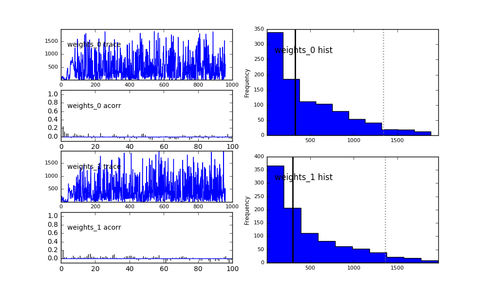
Since the variable weights is now a vector of floating point values, each
value gets its own plot and is denoted with the suffix _i, where i is
the index of the value. The template weight of model A is weights_0, the
weight of model B is weights_1.
Now let us see what the posterior looks like when we take the actual data into account:
mcmc = lm.mcmc(mixed_model)
mcmc.sample(iter=250000, burn=10000, tune_throughout=True, thin=250)
pymc.Matplot.plot(mcmc, suffix='_mixed')

Compare the 95% credible interval of weights_0 with the confidence interval
we constructed in a previous example.
PyMC will give you these 1D histograms for all parameters in your models. For two parameters, we can still plot everything into a single histogram though:
weights = mcmc.trace('weights')[:]
fig, ax = plt.subplots()
ax.hist2d(weights[:,0],weights[:,1], bins=20)
ax.set_xlabel("model A weight")
ax.set_ylabel("model B weight")
fig.savefig("posterior.png")
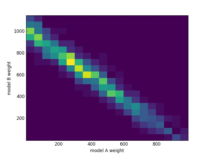
The preference for model B is quite clear. The trace contains all information about the posterior distribution of the model parameters, and we can do calculations with it. For example, let us take a look at the posterior probability of the sum of weights:
fig, ax = plt.subplots()
ax.hist(weights.sum(axis=1), bins=20)
ax.set_xlabel("sum of template weights")
fig.savefig("sum_posterior.png")

The response matrix (and thus the LikelihoodMachine) is only valid
for a certain range of values in the truth bins. If the tested theory predicts
more events than were simulated and used to build the matrix, the results are
not well predicted. It is thus necessary to test whether the posterior
distribution of the truth bin values as predicted by the models is far enough
away from those limits:
truth_trace = mixed_model.translate(weights)
toys = mcmc.trace('toy_index')[:]
lm.plot_truth_bin_traces("truth_traces.png", truth_trace, plot_limits='relative')
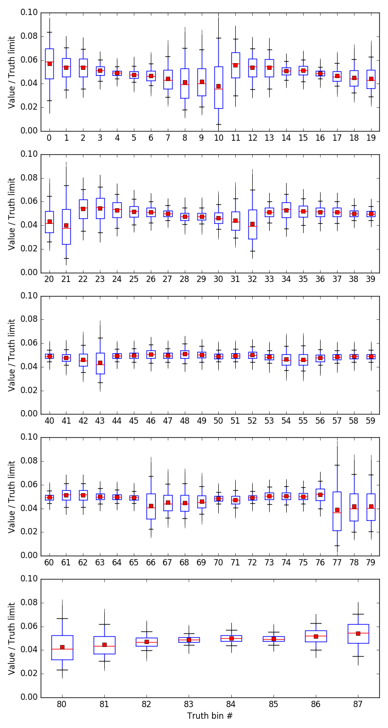
The box plots show the full range of the sample (vertical lines), the quartiles (boxes), the median (horizontal lines), 5% and 95% percentile (error bars), and the mean values (points). Here it is clear that the posterior distributions are much lower than the limits.
There is a similar method to plot the predicted expectation values in reco space:
lm.plot_reco_bin_traces("reco_traces.png", truth_trace, toy_index=toys, plot_data=True)

This can be used as a visual check of whether the models can cover the measured data at all.